TensorFlow Crash Course#


Readings: [RM19] [Keras API docs]
Introduction#
This notebook covers TF datasets, creating and training models with Keras, and internals such as static graphs and auto-differentiation using GradientTape. We also look into custom functionality such as modifying the train and eval step of the Keras fit function. A basic understanding of neural networks is assumed.
import os
import warnings
from pathlib import Path

import tensorflow as tf
import tensorflow.keras as kr
import tensorflow_datasets as tfds

import pandas as pd
import numpy as np
import seaborn as sns
import matplotlib.pyplot as plt
from matplotlib_inline import backend_inline


def set_random_seed(seed=0, deterministic=False):
    tf.keras.utils.set_random_seed(seed)
    if deterministic:
        tf.config.experimental.enable_op_determinism()


DATASET_DIR = Path("./data").absolute()
RANDOM_SEED = 42

warnings.simplefilter(action="ignore")
backend_inline.set_matplotlib_formats("svg")
set_random_seed(seed=RANDOM_SEED)

print(tf.__version__)
print(tf.config.list_physical_devices("GPU"))
2.10.0
[PhysicalDevice(name='/physical_device:GPU:0', device_type='GPU')]
os.environ["TF_CPP_MIN_LOG_LEVEL"] = "2"
TF Datasets#
TensorFlow provides the tf.data.Dataset API to facilitate efficient pipelines which support batching, shuffling, and mapping for loading and lazy preprocessing of input data. We can initialize a TF dataset from an existing tensor as follows:
a = tf.range(5)
ds = tf.data.Dataset.from_tensor_slices(a)
print(ds, "\n")

for item in ds:
    print(item)
Metal device set to: Apple M1

systemMemory: 8.00 GB
maxCacheSize: 2.67 GB

<TensorSliceDataset element_spec=TensorSpec(shape=(), dtype=tf.int32, name=None)>

tf.Tensor(0, shape=(), dtype=int32)
tf.Tensor(1, shape=(), dtype=int32)
tf.Tensor(2, shape=(), dtype=int32)
tf.Tensor(3, shape=(), dtype=int32)
tf.Tensor(4, shape=(), dtype=int32)
Batching#
Datasets supports batching of multiple tensors:
X = tf.random.uniform([10, 3], dtype=tf.float32)
y = tf.range(10)

ds = tf.data.Dataset.from_tensor_slices((X, y))
for x, t in ds.batch(3, drop_remainder=True):
    print(pd.DataFrame({
        "X1": x.numpy()[:, 0],
        "X2": x.numpy()[:, 1],
        "X3": x.numpy()[:, 2],
        "y": t.numpy()
    }), "\n")
         X1        X2        X3  y
0  0.664562  0.441007  0.352883  0
1  0.464483  0.033660  0.684672  1
2  0.740117  0.872445  0.226326  2

         X1        X2        X3  y
0  0.223197  0.310388  0.722336  3
1  0.133187  0.548064  0.574609  4
2  0.899683  0.009464  0.521231  5

         X1        X2        X3  y
0  0.634544  0.199328  0.729422  6
1  0.545835  0.107566  0.676706  7
2  0.660276  0.336950  0.601418  8
Dropping the remainder ensures all batches are of equal size.
Transformations#
Batch transformation can be done using map.
This also returns a Dataset object:
T = lambda x, y: (10 * x - 3, y)
dst = ds.map(T)
for x, y in dst.batch(3):
    print(pd.DataFrame({
        "X1": x.numpy()[:, 0],
        "X2": x.numpy()[:, 1],
        "X3": x.numpy()[:, 2],
        "y":  y.numpy()
    }), "\n")
         X1        X2        X3  y
0  3.645621  1.410068  0.528825  0
1  1.644825 -2.663396  3.846724  1
2  4.401175  5.724445 -0.736737  2

         X1        X2        X3  y
0 -0.768031  0.103881  4.223358  3
1 -1.668128  2.480639  2.746088  4
2  5.996835 -2.905363  2.212307  5

         X1        X2        X3  y
0  3.345445 -1.006717  4.294225  6
1  2.458345 -1.924345  3.767061  7
2  3.602763  0.369504  3.014176  8

         X1        X2        X3  y
0 -0.893742  5.527372  1.406218  9
Remark. Various optimizations such as prefetching, parallelism (Fig. 144), and caching exist for TF datasets. See TF docs. For example, the above map is inefficient since it applies the map on at a time instead of vectorized through a batch.

Fig. 144 Pre-pocessing steps overlap, reducing the overall time for a single iteration. Source#
Shuffle#
It is important to feed training data as randomly shuffled batches when training with SGD. Otherwise, the weight updates will be biased with regards to ordering of the input data. TensorFlow implements the .shuffle method on dataset objects with a buffer_size parameter for controlling the chunk size. This results in a tradeoff between shuffle quality and memory.
fig = plt.figure(figsize=(10, 4))
buffer_size = [1, 20, 60, 100]
for i in range(len(buffer_size)):
    shuffled_data = []
    ds_range = tf.data.Dataset.from_tensor_slices(tf.range(100))
    for x in ds_range.shuffle(buffer_size[i]).batch(1):
        shuffled_data.append(x.numpy()[0])

    ax = fig.add_subplot(1, 4, i+1)
    ax.bar(range(100), shuffled_data)
    ax.set_title(f"buffer_size={buffer_size[i]}")

plt.tight_layout()
plt.show()

A buffer_size of 1 is essentially the same dataset, while a buffer_size equal to the length of the dataset is a full shuffle. Note that the .shuffle returns a ShuffleDataset and has the argument reshuffle_each_iteration which defaults to True. This means that the resulting dataset reshuffles each time we iterate over it.
ds = tf.data.Dataset.range(3)
list(ds.shuffle(3).repeat(2).as_numpy_iterator())
[1, 2, 0, 2, 1, 0]
Setting it to False means that it is shuffled once, then it is fixed over iterations:
ds = tf.data.Dataset.range(3)
list(ds.shuffle(3, reshuffle_each_iteration=False).repeat(2).as_numpy_iterator())
[1, 2, 0, 1, 2, 0]
Creating epochs#
The shuffle, batch, repeat pattern generates epochs for neural network training:
num_epochs = 2
batch_size = 3
buffer_size = 6
for i in range(num_epochs):
    for x, t in dst.shuffle(buffer_size).batch(batch_size, drop_remainder=True):
        print(pd.DataFrame({
            "X1": x.numpy()[:, 0],
            "X2": x.numpy()[:, 1],
            "X3": x.numpy()[:, 2],
            "y": t.numpy()
        }), "\n")
         X1        X2        X3  y
0  5.996835 -2.905363  2.212307  5
1 -0.768031  0.103881  4.223358  3
2  3.345445 -1.006717  4.294225  6

         X1        X2        X3  y
0 -1.668128  2.480639  2.746088  4
1  4.401175  5.724445 -0.736737  2
2  3.602763  0.369504  3.014176  8

         X1        X2        X3  y
0  3.645621  1.410068  0.528825  0
1  2.458345 -1.924345  3.767061  7
2  1.644825 -2.663396  3.846724  1

         X1        X2        X3  y
0  1.644825 -2.663396  3.846724  1
1  3.345445 -1.006717  4.294225  6
2 -1.668128  2.480639  2.746088  4

         X1        X2        X3  y
0  3.602763  0.369504  3.014176  8
1 -0.893742  5.527372  1.406218  9
2 -0.768031  0.103881  4.223358  3

         X1        X2        X3  y
0  2.458345 -1.924345  3.767061  7
1  4.401175  5.724445 -0.736737  2
2  3.645621  1.410068  0.528825  0
From local files#
Transformations can be used with any user-defined function. For example, we can load data from disk by creating a TF dataset of filenames. Then, we can define a map that loads the files from disk:
from functools import partial

# Define mapping function: (filename, label) -> (RGB array, label)
def load_and_preprocess(path, label, img_width=124, img_height=124):
    img_raw = tf.io.read_file(path)
    img = tf.image.decode_jpeg(img_raw, channels=3)
    img = tf.image.resize(img, [img_height, img_width])
    img /= 255.0
    return img, label


# File list
DATASET_DIR = Path("./tf-course/data").absolute()
cat_path = DATASET_DIR / "cat2dog" / "cat2dog" / "trainA"
dog_path = DATASET_DIR / "cat2dog" / "cat2dog" / "trainB"
cat_files = sorted([str(path) for path in cat_path.glob("*.jpg")])
dog_files = sorted([str(path) for path in dog_path.glob("*.jpg")])

# Create dataset of RGB arrays resized to 32x32x3
X = cat_files + dog_files
y = [0] * len(cat_files) + [1] * len(dog_files)
ds_filenames = tf.data.Dataset.from_tensor_slices((X, y))
ds_images = ds_filenames.map(partial(load_and_preprocess, img_width=32, img_height=32))

# Display one image and its label (0 = cat, 1 = dog)
img, label = next(iter(ds_images.shuffle(len(ds_images)).batch(6)))
fig, ax = plt.subplots(1, 6, figsize=(12, 2))
for i in range(6):
    ax[i].imshow(img[i, :, :, :])
    ax[i].set_title(int(label[i]))

Mechanics of TF#
For advanced deep learning models, we need lower-level features of TensorFlow. This allows accessing and modifying layer weights and gradients, performing autodiff, and creating more efficient static computation graphs from ordinary Python code. This sections takes a brief look into the @tf.function decorator and performing autograd (of arbitrary order) with GradientTape.
Static graph execution#
Computations with eager execution are not as efficient as the static graph execution which is precompiled. TensorFlow provides a simple mechanism for compiling a normal Python function f to a static graph by using tf.function(f) or use the @tf.function decorator in the definition of f.
def f(x, y, z):
    return x + y + z

f_graph = tf.function(f)
tf.print("Scalar Inputs:", f_graph(1, 2, 3))
tf.print("Rank 1 Inputs:", f_graph([1], [2], [3]))
tf.print("Rank 2 Inputs:", f_graph([[1]], [[2]], [[3]]))
Scalar Inputs: 6
Rank 1 Inputs: [1, 2, 3]
Rank 2 Inputs: [[1], [2], [3]]
Here we encounter a first subtlety with static graphs. The above three executions actually create three graphs under the hood. TensorFlow uses a tracing mechanism to construct a graph based on the input arguments. For this tracing mechanism, TensorFlow generates a tuple of keys based on the input signatures given for calling the function. The generated keys are as follows:
For
tf.Tensorarguments, the key is based on their shapes anddtypes.For Python types, such as lists, their
id()is used to generate cache keys.For Python primitive values, the cache keys are based on the input values.
Upon calling a decorated function, TF either retrieves the graph by key or creates one if the key does not exist. Graph creation includes TensorFlow as well as Python operations as nodes. See here for details. This is not generally an issue in practice where the shape of the input is expected. To limit input signature and types:
f_graph = tf.function(f, input_signature=(
    tf.TensorSpec(shape=[None], dtype=tf.int32),
    tf.TensorSpec(shape=[None], dtype=tf.int32),
    tf.TensorSpec(shape=[None], dtype=tf.int32),
))

f_graph([1], [2], [3])
<tf.Tensor: shape=(1,), dtype=int32, numpy=array([6], dtype=int32)>
try:
    f_graph(1, 2, 3)
except Exception as e:
    print(e)
Python inputs incompatible with input_signature:
  inputs: (
    1,
    2,
    3)
  input_signature: (
    TensorSpec(shape=(None,), dtype=tf.int32, name=None),
    TensorSpec(shape=(None,), dtype=tf.int32, name=None),
    TensorSpec(shape=(None,), dtype=tf.int32, name=None)).
Timing static graphs#
import matplotlib.pyplot as plt
import numpy as np
from timeit import timeit

def compare_timings(f, x, n):
    # Define functions
    eager_function = f
    graph_function = tf.function(f)

    # Timing
    graph_time = timeit(lambda: graph_function(*x), number=n) / n
    eager_time = timeit(lambda: eager_function(*x), number=n) / n

    return {
        "graph": graph_time,
        "eager": eager_time
    }

# sample input
u = tf.random.uniform([256, 28, 28])
Comparing static graph execution with eager execution on a dense network:
from tensorflow.keras.layers import Flatten, Dense

model = kr.Sequential()
model.add(Flatten())
model.add(Dense(256, "relu"))
model.add(Dense(10, "softmax"))

dense_times = compare_timings(model, [u], n=10000);
Convolution operation:
from tensorflow.keras.layers import Conv2D, AveragePooling2D

conv_model = kr.Sequential()
conv_model.add(Conv2D(filters=6, kernel_size=(3, 3), activation="relu", input_shape=(28, 28, 1)))
conv_model.add(Conv2D(filters=6, kernel_size=(3, 3), activation="relu", input_shape=(28, 28, 1)))
conv_model.add(AveragePooling2D())

conv_times = compare_timings(conv_model, [u], n=10000);
Results:
Show code cell source
models = ["dense", "conv"]
eager = [eval(m + "_times")["eager"] / eval(m + "_times")["eager"] for m in models]
graph = [eval(m + "_times")["graph"] / eval(m + "_times")["eager"] for m in models]
x = np.arange(len(models))

plt.figure(figsize=(8, 5))
plt.grid(linestyle="dotted", zorder=1)
plt.bar(x + 0.1, eager, width=0.2, label="eager", zorder=3)
plt.bar(x - 0.1, graph, width=0.2, label="graph", zorder=3)
plt.xticks(x, models)
plt.ylabel(r"% eager time")
plt.ylim(0, 1.2)
plt.legend();

The above results (sorted in decreasing no. of parameters) show that graph execution can be faster can be faster than eager code, especially for graphs with expensive operations. But for graphs with fewer expensive operations (like convolutions), you may see little speedup or even worse with cheap operations due to the overhead of tracing.
Remark. For example, the following error message highlights cases where we make inefficient use of tracing. Recall the rules above for generating keys for static graphs based on the input. This guide on tracing mechanism is also helpful.
WARNING:tensorflow:6 out of the last 6 calls to <keras.engine.sequential.Sequential object at 0x28575dfa0> triggered tf.function retracing. Tracing is expensive and the excessive number of tracings could be due to (1) creating @tf.function repeatedly in a loop, (2) passing tensors with different shapes, (3) passing Python objects instead of tensors. For (1), please define your @tf.function outside of the loop.
TF variables#
A variable maintains shared, persistent state that implements the concept of model parameter in TensorFlow. TF modules are essentially named containers for variables and implements a forward method. Below we implement a linear layer in TF:
class MyModule(tf.Module):
    def __init__(self):
        init = kr.initializers.GlorotNormal()
        self.a = tf.Variable(-1.0, trainable=False)
        self.w = tf.Variable(init(shape=(3, 2)), trainable=True)
        self.b = tf.Variable(init(shape=(1, 2)), trainable=True)

    def __call__(self, x):
        return  self.a * x @ self.w + self.b


m = MyModule()
print("All variables:")
[print(v.shape) for v in m.variables]

print("\nTrainable:")
[print(v.shape) for v in m.trainable_variables];
All variables:
()
(1, 2)
(3, 2)

Trainable:
(1, 2)
(3, 2)
Testing call method:
bs = 6
x = tf.random.uniform([bs, 3], dtype=tf.float32)
m(x)
<tf.Tensor: shape=(6, 2), dtype=float32, numpy=
array([[ 0.10170744, -0.2540003 ],
       [ 0.09207833,  0.00356225],
       [ 0.08909164,  0.0276397 ],
       [ 0.04640259, -0.02139331],
       [ 0.10501287, -0.23698108],
       [ 0.15016323, -0.22649907]], dtype=float32)>
Updating variables (see other ops):
m.w.assign_add(100.0 * tf.ones_like(m.w))
m(x)
<tf.Tensor: shape=(6, 2), dtype=float32, numpy=
array([[-223.61987 , -223.97559 ],
       [ -24.395416,  -24.483934],
       [ -95.51543 ,  -95.57688 ],
       [-107.76779 , -107.83559 ],
       [-215.19844 , -215.54044 ],
       [-131.50824 , -131.8849  ]], dtype=float32)>
Autograd with GradientTape#
TensorFlow supports automatic differentiation for operations defined in the language. For nested functions, TF provides a context called GradientTape for calculating gradients of these computed tensors with respect to its dependent nodes in the computation graph. This allows TensorFlow to trace the graph forwards to make predictions and backwards to compute the weight gradients.
# scope outside tf.GradientTape
w = tf.Variable(1.0)
b = tf.Variable(0.5)

# data
x = tf.convert_to_tensor([1.4])
y = tf.convert_to_tensor([2.1])

with tf.GradientTape() as tape:
    z = tf.add(tf.multiply(w, x), b)
    loss = tf.reduce_sum(tf.square(y - z))

grad = tape.gradient(loss, w)
tf.print("∂(loss)/∂w =", grad)
tf.print(2 * (y - w*x - b) * (-x)) # symbolic
∂(loss)/∂w = -0.559999764
[-0.559999764]
It turns out that TF supports stacking gradient tapes which allow us to compute higher order derivatives:
with tf.GradientTape() as outer_tape:
    with tf.GradientTape() as inner_tape:
        z = tf.add(tf.multiply(w, x), b)
        loss = tf.reduce_sum(tf.square(y - z))
    grad_w = inner_tape.gradient(loss, w)
grad_wb = outer_tape.gradient(grad_w, b)

tf.print("∂²(loss)/∂w∂b =", grad_wb)
tf.print(2 * (-1) * (-x)) # symbolic
∂²(loss)/∂w∂b = 2.8
[2.8]
For non-trainable variables and other Tensor objects, we have to manually add them using tape.watch().
with tf.GradientTape() as tape:
    tape.watch(x) # <-
    z = tf.add(tf.multiply(w, x), b)
    loss = tf.reduce_sum(tf.square(y - z))

grad = tape.gradient(loss, x)
tf.print("∂(loss)/∂x =", grad)
tf.print(2 * (y - w*x - b) * (-w)) # check symbolic
∂(loss)/∂x = [-0.399999857]
[-0.399999857]
Note that the tape will keep the resources only for a single gradient computation by default. So after calling tape.gradient() once, the resources are released. If we want to compute more than one gradient, we need to persist it.
with tf.GradientTape(persistent=True) as tape:
    tape.watch(x)
    z = tf.add(tf.multiply(w, x), b)
    loss = tf.reduce_sum(tf.square(y - z))

tf.print("∂(loss)/∂w =", tape.gradient(loss, w))
tf.print("∂(loss)/∂x =", tape.gradient(loss, x)) # error if not persisted
∂(loss)/∂w = -0.559999764
∂(loss)/∂x = [-0.399999857]
SGD step update#
During SGD, we are computing gradients of a loss term with respect to model weights, which we use to update the weights according to some rule defined by an optimization algorithm. For Keras optimizers, we can do this by using .apply_gradients:
grad_w = tape.gradient(loss, w)
grad_b = tape.gradient(loss, b)
lr = 0.1
tf.print("w =", w)
tf.print("b =", b)
tf.print("λ =", lr)
tf.print("grad_[w, b] =", [grad_w, grad_b])

# Define keras optimizer; apply optimizer step
optimizer = kr.optimizers.SGD(learning_rate=lr)
optimizer.apply_gradients(zip([grad_w, grad_b], [w, b]))

# Print updates
tf.print()
tf.print("w - λ·∂(loss)/∂w ≟", w)
tf.print("b - λ·∂(loss)/∂b ≟", b)
w = 1
b = 0.5
λ = 0.1
grad_[w, b] = [-0.559999764, -0.399999857]

w - λ·∂(loss)/∂w ≟ 1.056
b - λ·∂(loss)/∂b ≟ 0.539999962
Checks out.
Model training#
Keras provides multiple layers of abstraction to make the implementation of standard architectures very convenient. This allows us to implement custom functionality, such as neural network layers, which is very useful in research projects. The tradeoff with ease of use is that Keras code can be significantly slower due to large overhead. We will explore how to implement more efficient minimal custom training loops.
How to build your models#
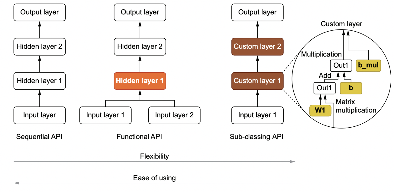
Fig. 145 Sequential, functional, and sub-classing APIs for creating models.#
Sequential#
For models that perform sequential transforms on input data, we typically use kr.Sequential(). Layers can then be added using the add() method. Alternatively, we can pass a list of Keras layers in the constructor.
model = kr.Sequential()
model.add(Dense(units=16, activation="relu"))
model.add(Dense(units=32, activation="relu"))
model.add(Dense(units=1,  activation="relu"))

# Build model
model.build(input_shape=(None, 4))
model.summary()
Model: "sequential_2"
_________________________________________________________________
 Layer (type)                Output Shape              Param #
=================================================================
 dense_2 (Dense)             (None, 16)                80

 dense_3 (Dense)             (None, 32)                544

 dense_4 (Dense)             (None, 1)                 33

=================================================================
Total params: 657
Trainable params: 657
Non-trainable params: 0
_________________________________________________________________
for v in model.variables:
    print(f"{v.name:20s} {str(v.trainable):7} {v.shape}")
dense_2/kernel:0     True    (4, 16)
dense_2/bias:0       True    (16,)
dense_3/kernel:0     True    (16, 32)
dense_3/bias:0       True    (32,)
dense_4/kernel:0     True    (32, 1)
dense_4/bias:0       True    (1,)
Functional#
Not all architectures involve sequential transformation. Keras’ functional API comes in handy for more complex transformations such as residual connections. Observe that the model build adds a new layer called tf.__operators__.add under the hood:
# Specify input and output
x = kr.Input(shape=(2,))
f = Dense(units=2, input_shape=(2,), activation="relu")(x)
out = Dense(units=1, activation="sigmoid")(x + f)

# Build model
model = kr.Model(inputs=x, outputs=out)
model.summary() # compile, fit, etc. also works
Model: "model"
__________________________________________________________________________________________________
 Layer (type)                   Output Shape         Param #     Connected to
==================================================================================================
 input_1 (InputLayer)           [(None, 2)]          0           []

 dense_5 (Dense)                (None, 2)            6           ['input_1[0][0]']

 tf.__operators__.add (TFOpLamb  (None, 2)           0           ['input_1[0][0]',
 da)                                                              'dense_5[0][0]']

 dense_6 (Dense)                (None, 1)            3           ['tf.__operators__.add[0][0]']

==================================================================================================
Total params: 9
Trainable params: 9
Non-trainable params: 0
__________________________________________________________________________________________________
Model class#
To have fine-grained control when building more complex models, we can subclass kr.Model. This allows us to define __init__ for initializing model parameters, and the call method for defining forward pass. The subclass inherits methods such as build(), compile(), and fit() which means the usual Keras methods work instances of this class.
class MyModel(kr.Model):
    def __init__(self):
        super().__init__()
        self.dense1 = Dense(units=128, activation="tanh")
        self.dense2 = Dense(units=10, activation="sigmoid")

    def call(self, x):
        h1 = self.dense1(x)
        out = self.dense2(h1)
        return out


# Build model and model summary
model = MyModel()
model.build(input_shape=(None, 2))
model.summary()
Model: "my_model"
_________________________________________________________________
 Layer (type)                Output Shape              Param #
=================================================================
 dense_7 (Dense)             multiple                  384

 dense_8 (Dense)             multiple                  1290

=================================================================
Total params: 1,674
Trainable params: 1,674
Non-trainable params: 0
_________________________________________________________________
Solving the XOR problem#
The XOR is the smallest dataset that is not linearly separable (also the most historically interesting relative to its size [Min69]). Our version of the XOR dataset is generated by adding Gaussian noise to points (-1, -1), (-1, 1), (1, -1) and (1, 1). Points generated from (1, 1) and (-1, -1) will be labeled 1 otherwise 0. A dataset of size 200 points will be generated with half used for validation.
# Create dataset
X = []
Y = []
for p in [(1, 1), (-1, -1), (-1, 1), (1, -1)]:
    x = np.array(p) + np.random.normal(0, 0.3, size=(50, 2))
    y = int(p[0] * p[1] > 0) * np.ones(50)
    X.append(x)
    Y.append(y)

X = np.concatenate(X)
Y = np.concatenate(Y)

# Train-test split
indices = list(range(200))
np.random.shuffle(indices)
valid = indices[:100]
train = indices[100:]
X_valid, y_valid = X[valid, :], Y[valid]
X_train, y_train = X[train, :], Y[train]

# Visualize dataset
fig = plt.figure(figsize=(6, 6))
plt.scatter(X_train[y_train==0, 0], X_train[y_train==0, 1], s=40, edgecolor="black", label=0)
plt.scatter(X_train[y_train==1, 0], X_train[y_train==1, 1], s=40, edgecolor="black", label=1)
plt.legend();

From the geometry of the dataset, we have to use a network that has at least depth 2, so that the network is not a linear classifier. However, since the dataset is small, we want the network to be not too wide (and not too deep), so the model does not overfit the dataset. Our XOR model only has <20 parameters.
model = kr.Sequential()
model.add(kr.layers.Dense(units=4, activation="tanh"))
model.add(kr.layers.Dense(units=1,  activation="sigmoid"))

model.build(input_shape=(None, 2))
model.summary()
Model: "sequential_3"
_________________________________________________________________
 Layer (type)                Output Shape              Param #
=================================================================
 dense_9 (Dense)             (None, 4)                 12

 dense_10 (Dense)            (None, 1)                 5

=================================================================
Total params: 17
Trainable params: 17
Non-trainable params: 0
_________________________________________________________________
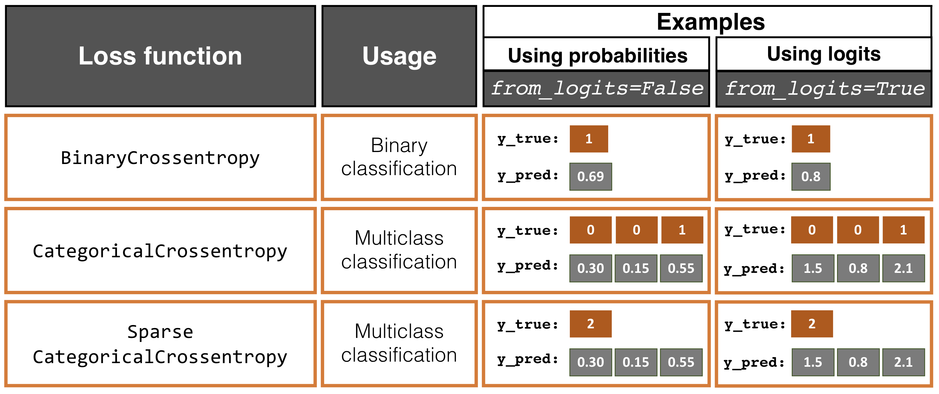
Remark. The default behavior in Keras is from_logits=False where the expected network output are class-probabilities in [0, 1] over the number of classes that sum to 1.0. This can come from a softmax activation, though any output is allowed as long as the outputs are class distributions. Here the loss function computes -log q[k*] where q is the output of the network and k* is the index of the true class. Predictions of class label can be obtained using tf.argmax(q).
Model training:
model.compile(
    optimizer=kr.optimizers.SGD(),
    loss=kr.losses.BinaryCrossentropy(from_logits=False),
    metrics=[kr.metrics.BinaryAccuracy()]
)

hist = model.fit(
    X_train, y_train,
    validation_data=(X_valid, y_valid),
    epochs=120,
    batch_size=2, verbose=1
)
Show code cell output
Epoch 1/120
50/50 [==============================] - 4s 17ms/step - loss: 0.6812 - binary_accuracy: 0.5700 - val_loss: 0.7189 - val_binary_accuracy: 0.5100
Epoch 2/120
50/50 [==============================] - 1s 12ms/step - loss: 0.6720 - binary_accuracy: 0.6000 - val_loss: 0.7120 - val_binary_accuracy: 0.5500
Epoch 3/120
50/50 [==============================] - 1s 12ms/step - loss: 0.6641 - binary_accuracy: 0.6600 - val_loss: 0.7053 - val_binary_accuracy: 0.6300
Epoch 4/120
50/50 [==============================] - 1s 12ms/step - loss: 0.6562 - binary_accuracy: 0.7300 - val_loss: 0.6990 - val_binary_accuracy: 0.7000
Epoch 5/120
50/50 [==============================] - 1s 12ms/step - loss: 0.6484 - binary_accuracy: 0.7800 - val_loss: 0.6913 - val_binary_accuracy: 0.7000
Epoch 6/120
50/50 [==============================] - 1s 11ms/step - loss: 0.6404 - binary_accuracy: 0.7900 - val_loss: 0.6832 - val_binary_accuracy: 0.7000
Epoch 7/120
50/50 [==============================] - 1s 11ms/step - loss: 0.6315 - binary_accuracy: 0.7900 - val_loss: 0.6739 - val_binary_accuracy: 0.7000
Epoch 8/120
50/50 [==============================] - 1s 14ms/step - loss: 0.6228 - binary_accuracy: 0.7800 - val_loss: 0.6643 - val_binary_accuracy: 0.7000
Epoch 9/120
50/50 [==============================] - 1s 12ms/step - loss: 0.6124 - binary_accuracy: 0.7900 - val_loss: 0.6542 - val_binary_accuracy: 0.7000
Epoch 10/120
50/50 [==============================] - 1s 11ms/step - loss: 0.6024 - binary_accuracy: 0.7900 - val_loss: 0.6427 - val_binary_accuracy: 0.7000
Epoch 11/120
50/50 [==============================] - 1s 11ms/step - loss: 0.5912 - binary_accuracy: 0.7900 - val_loss: 0.6305 - val_binary_accuracy: 0.7000
Epoch 12/120
50/50 [==============================] - 1s 12ms/step - loss: 0.5798 - binary_accuracy: 0.7900 - val_loss: 0.6177 - val_binary_accuracy: 0.7000
Epoch 13/120
50/50 [==============================] - 1s 12ms/step - loss: 0.5677 - binary_accuracy: 0.7900 - val_loss: 0.6038 - val_binary_accuracy: 0.7000
Epoch 14/120
50/50 [==============================] - 1s 11ms/step - loss: 0.5552 - binary_accuracy: 0.7900 - val_loss: 0.5890 - val_binary_accuracy: 0.7000
Epoch 15/120
50/50 [==============================] - 1s 12ms/step - loss: 0.5422 - binary_accuracy: 0.7900 - val_loss: 0.5742 - val_binary_accuracy: 0.7000
Epoch 16/120
50/50 [==============================] - 1s 13ms/step - loss: 0.5288 - binary_accuracy: 0.7900 - val_loss: 0.5592 - val_binary_accuracy: 0.7000
Epoch 17/120
50/50 [==============================] - 1s 13ms/step - loss: 0.5155 - binary_accuracy: 0.8000 - val_loss: 0.5440 - val_binary_accuracy: 0.7000
Epoch 18/120
50/50 [==============================] - 1s 16ms/step - loss: 0.5016 - binary_accuracy: 0.8000 - val_loss: 0.5286 - val_binary_accuracy: 0.7000
Epoch 19/120
50/50 [==============================] - 1s 13ms/step - loss: 0.4876 - binary_accuracy: 0.8000 - val_loss: 0.5129 - val_binary_accuracy: 0.7400
Epoch 20/120
50/50 [==============================] - 1s 12ms/step - loss: 0.4739 - binary_accuracy: 0.8100 - val_loss: 0.4974 - val_binary_accuracy: 0.7600
Epoch 21/120
50/50 [==============================] - 1s 13ms/step - loss: 0.4607 - binary_accuracy: 0.8100 - val_loss: 0.4815 - val_binary_accuracy: 0.8200
Epoch 22/120
50/50 [==============================] - 1s 14ms/step - loss: 0.4472 - binary_accuracy: 0.8300 - val_loss: 0.4665 - val_binary_accuracy: 0.8600
Epoch 23/120
50/50 [==============================] - 1s 12ms/step - loss: 0.4338 - binary_accuracy: 0.8400 - val_loss: 0.4513 - val_binary_accuracy: 0.9000
Epoch 24/120
50/50 [==============================] - 1s 14ms/step - loss: 0.4209 - binary_accuracy: 0.8900 - val_loss: 0.4367 - val_binary_accuracy: 0.9100
Epoch 25/120
50/50 [==============================] - 1s 15ms/step - loss: 0.4082 - binary_accuracy: 0.9200 - val_loss: 0.4226 - val_binary_accuracy: 0.9300
Epoch 26/120
50/50 [==============================] - 1s 15ms/step - loss: 0.3952 - binary_accuracy: 0.9300 - val_loss: 0.4090 - val_binary_accuracy: 0.9300
Epoch 27/120
50/50 [==============================] - 1s 16ms/step - loss: 0.3834 - binary_accuracy: 0.9400 - val_loss: 0.3960 - val_binary_accuracy: 0.9400
Epoch 28/120
50/50 [==============================] - 1s 15ms/step - loss: 0.3716 - binary_accuracy: 0.9400 - val_loss: 0.3832 - val_binary_accuracy: 0.9400
Epoch 29/120
50/50 [==============================] - 1s 13ms/step - loss: 0.3600 - binary_accuracy: 0.9400 - val_loss: 0.3705 - val_binary_accuracy: 0.9500
Epoch 30/120
50/50 [==============================] - 1s 15ms/step - loss: 0.3492 - binary_accuracy: 0.9600 - val_loss: 0.3585 - val_binary_accuracy: 0.9500
Epoch 31/120
50/50 [==============================] - 1s 14ms/step - loss: 0.3387 - binary_accuracy: 0.9800 - val_loss: 0.3473 - val_binary_accuracy: 0.9600
Epoch 32/120
50/50 [==============================] - 1s 14ms/step - loss: 0.3284 - binary_accuracy: 0.9800 - val_loss: 0.3359 - val_binary_accuracy: 0.9700
Epoch 33/120
50/50 [==============================] - 1s 13ms/step - loss: 0.3185 - binary_accuracy: 0.9800 - val_loss: 0.3252 - val_binary_accuracy: 0.9700
Epoch 34/120
50/50 [==============================] - 1s 13ms/step - loss: 0.3090 - binary_accuracy: 0.9900 - val_loss: 0.3151 - val_binary_accuracy: 0.9700
Epoch 35/120
50/50 [==============================] - 1s 12ms/step - loss: 0.2999 - binary_accuracy: 0.9900 - val_loss: 0.3053 - val_binary_accuracy: 0.9900
Epoch 36/120
50/50 [==============================] - 1s 12ms/step - loss: 0.2911 - binary_accuracy: 0.9900 - val_loss: 0.2959 - val_binary_accuracy: 1.0000
Epoch 37/120
50/50 [==============================] - 1s 12ms/step - loss: 0.2825 - binary_accuracy: 0.9900 - val_loss: 0.2870 - val_binary_accuracy: 1.0000
Epoch 38/120
50/50 [==============================] - 1s 14ms/step - loss: 0.2743 - binary_accuracy: 0.9900 - val_loss: 0.2783 - val_binary_accuracy: 1.0000
Epoch 39/120
50/50 [==============================] - 1s 15ms/step - loss: 0.2666 - binary_accuracy: 0.9900 - val_loss: 0.2701 - val_binary_accuracy: 1.0000
Epoch 40/120
50/50 [==============================] - 1s 15ms/step - loss: 0.2590 - binary_accuracy: 0.9900 - val_loss: 0.2624 - val_binary_accuracy: 1.0000
Epoch 41/120
50/50 [==============================] - 1s 15ms/step - loss: 0.2518 - binary_accuracy: 0.9900 - val_loss: 0.2549 - val_binary_accuracy: 1.0000
Epoch 42/120
50/50 [==============================] - 1s 14ms/step - loss: 0.2451 - binary_accuracy: 0.9900 - val_loss: 0.2477 - val_binary_accuracy: 1.0000
Epoch 43/120
50/50 [==============================] - 1s 15ms/step - loss: 0.2382 - binary_accuracy: 0.9900 - val_loss: 0.2409 - val_binary_accuracy: 1.0000
Epoch 44/120
50/50 [==============================] - 1s 13ms/step - loss: 0.2320 - binary_accuracy: 0.9900 - val_loss: 0.2343 - val_binary_accuracy: 1.0000
Epoch 45/120
50/50 [==============================] - 1s 13ms/step - loss: 0.2258 - binary_accuracy: 0.9900 - val_loss: 0.2278 - val_binary_accuracy: 1.0000
Epoch 46/120
50/50 [==============================] - 1s 13ms/step - loss: 0.2200 - binary_accuracy: 0.9900 - val_loss: 0.2219 - val_binary_accuracy: 1.0000
Epoch 47/120
50/50 [==============================] - 1s 12ms/step - loss: 0.2144 - binary_accuracy: 0.9900 - val_loss: 0.2160 - val_binary_accuracy: 1.0000
Epoch 48/120
50/50 [==============================] - 1s 15ms/step - loss: 0.2091 - binary_accuracy: 0.9900 - val_loss: 0.2105 - val_binary_accuracy: 1.0000
Epoch 49/120
50/50 [==============================] - 1s 13ms/step - loss: 0.2039 - binary_accuracy: 0.9900 - val_loss: 0.2053 - val_binary_accuracy: 1.0000
Epoch 50/120
50/50 [==============================] - 1s 12ms/step - loss: 0.1989 - binary_accuracy: 1.0000 - val_loss: 0.2002 - val_binary_accuracy: 1.0000
Epoch 51/120
50/50 [==============================] - 1s 13ms/step - loss: 0.1941 - binary_accuracy: 1.0000 - val_loss: 0.1953 - val_binary_accuracy: 1.0000
Epoch 52/120
50/50 [==============================] - 1s 14ms/step - loss: 0.1896 - binary_accuracy: 1.0000 - val_loss: 0.1906 - val_binary_accuracy: 1.0000
Epoch 53/120
50/50 [==============================] - 1s 14ms/step - loss: 0.1852 - binary_accuracy: 1.0000 - val_loss: 0.1861 - val_binary_accuracy: 1.0000
Epoch 54/120
50/50 [==============================] - 1s 14ms/step - loss: 0.1809 - binary_accuracy: 1.0000 - val_loss: 0.1817 - val_binary_accuracy: 1.0000
Epoch 55/120
50/50 [==============================] - 1s 12ms/step - loss: 0.1768 - binary_accuracy: 1.0000 - val_loss: 0.1775 - val_binary_accuracy: 1.0000
Epoch 56/120
50/50 [==============================] - 1s 13ms/step - loss: 0.1730 - binary_accuracy: 1.0000 - val_loss: 0.1735 - val_binary_accuracy: 1.0000
Epoch 57/120
50/50 [==============================] - 1s 15ms/step - loss: 0.1692 - binary_accuracy: 1.0000 - val_loss: 0.1696 - val_binary_accuracy: 1.0000
Epoch 58/120
50/50 [==============================] - 1s 13ms/step - loss: 0.1655 - binary_accuracy: 1.0000 - val_loss: 0.1660 - val_binary_accuracy: 1.0000
Epoch 59/120
50/50 [==============================] - 1s 13ms/step - loss: 0.1620 - binary_accuracy: 1.0000 - val_loss: 0.1625 - val_binary_accuracy: 1.0000
Epoch 60/120
50/50 [==============================] - 1s 12ms/step - loss: 0.1586 - binary_accuracy: 1.0000 - val_loss: 0.1591 - val_binary_accuracy: 1.0000
Epoch 61/120
50/50 [==============================] - 1s 15ms/step - loss: 0.1555 - binary_accuracy: 1.0000 - val_loss: 0.1558 - val_binary_accuracy: 1.0000
Epoch 62/120
50/50 [==============================] - 1s 12ms/step - loss: 0.1522 - binary_accuracy: 1.0000 - val_loss: 0.1527 - val_binary_accuracy: 1.0000
Epoch 63/120
50/50 [==============================] - 1s 13ms/step - loss: 0.1493 - binary_accuracy: 1.0000 - val_loss: 0.1496 - val_binary_accuracy: 1.0000
Epoch 64/120
50/50 [==============================] - 1s 14ms/step - loss: 0.1463 - binary_accuracy: 1.0000 - val_loss: 0.1467 - val_binary_accuracy: 1.0000
Epoch 65/120
50/50 [==============================] - 1s 14ms/step - loss: 0.1435 - binary_accuracy: 1.0000 - val_loss: 0.1439 - val_binary_accuracy: 1.0000
Epoch 66/120
50/50 [==============================] - 1s 13ms/step - loss: 0.1408 - binary_accuracy: 1.0000 - val_loss: 0.1411 - val_binary_accuracy: 1.0000
Epoch 67/120
50/50 [==============================] - 1s 11ms/step - loss: 0.1381 - binary_accuracy: 1.0000 - val_loss: 0.1385 - val_binary_accuracy: 1.0000
Epoch 68/120
50/50 [==============================] - 1s 11ms/step - loss: 0.1356 - binary_accuracy: 1.0000 - val_loss: 0.1360 - val_binary_accuracy: 1.0000
Epoch 69/120
50/50 [==============================] - 1s 13ms/step - loss: 0.1331 - binary_accuracy: 1.0000 - val_loss: 0.1335 - val_binary_accuracy: 1.0000
Epoch 70/120
50/50 [==============================] - 1s 16ms/step - loss: 0.1307 - binary_accuracy: 1.0000 - val_loss: 0.1311 - val_binary_accuracy: 1.0000
Epoch 71/120
50/50 [==============================] - 1s 11ms/step - loss: 0.1284 - binary_accuracy: 1.0000 - val_loss: 0.1288 - val_binary_accuracy: 1.0000
Epoch 72/120
50/50 [==============================] - 1s 11ms/step - loss: 0.1262 - binary_accuracy: 1.0000 - val_loss: 0.1266 - val_binary_accuracy: 1.0000
Epoch 73/120
50/50 [==============================] - 1s 14ms/step - loss: 0.1240 - binary_accuracy: 1.0000 - val_loss: 0.1245 - val_binary_accuracy: 1.0000
Epoch 74/120
50/50 [==============================] - 1s 13ms/step - loss: 0.1218 - binary_accuracy: 1.0000 - val_loss: 0.1224 - val_binary_accuracy: 1.0000
Epoch 75/120
50/50 [==============================] - 1s 13ms/step - loss: 0.1199 - binary_accuracy: 1.0000 - val_loss: 0.1204 - val_binary_accuracy: 1.0000
Epoch 76/120
50/50 [==============================] - 1s 12ms/step - loss: 0.1179 - binary_accuracy: 1.0000 - val_loss: 0.1184 - val_binary_accuracy: 1.0000
Epoch 77/120
50/50 [==============================] - 1s 13ms/step - loss: 0.1161 - binary_accuracy: 1.0000 - val_loss: 0.1166 - val_binary_accuracy: 1.0000
Epoch 78/120
50/50 [==============================] - 1s 14ms/step - loss: 0.1141 - binary_accuracy: 1.0000 - val_loss: 0.1147 - val_binary_accuracy: 1.0000
Epoch 79/120
50/50 [==============================] - 1s 18ms/step - loss: 0.1124 - binary_accuracy: 1.0000 - val_loss: 0.1129 - val_binary_accuracy: 1.0000
Epoch 80/120
50/50 [==============================] - 1s 16ms/step - loss: 0.1106 - binary_accuracy: 1.0000 - val_loss: 0.1112 - val_binary_accuracy: 1.0000
Epoch 81/120
50/50 [==============================] - 1s 12ms/step - loss: 0.1089 - binary_accuracy: 1.0000 - val_loss: 0.1095 - val_binary_accuracy: 1.0000
Epoch 82/120
50/50 [==============================] - 1s 12ms/step - loss: 0.1073 - binary_accuracy: 1.0000 - val_loss: 0.1079 - val_binary_accuracy: 1.0000
Epoch 83/120
50/50 [==============================] - 1s 11ms/step - loss: 0.1057 - binary_accuracy: 1.0000 - val_loss: 0.1063 - val_binary_accuracy: 1.0000
Epoch 84/120
50/50 [==============================] - 1s 13ms/step - loss: 0.1041 - binary_accuracy: 1.0000 - val_loss: 0.1048 - val_binary_accuracy: 1.0000
Epoch 85/120
50/50 [==============================] - 1s 12ms/step - loss: 0.1026 - binary_accuracy: 1.0000 - val_loss: 0.1033 - val_binary_accuracy: 1.0000
Epoch 86/120
50/50 [==============================] - 1s 12ms/step - loss: 0.1011 - binary_accuracy: 1.0000 - val_loss: 0.1018 - val_binary_accuracy: 1.0000
Epoch 87/120
50/50 [==============================] - 1s 11ms/step - loss: 0.0997 - binary_accuracy: 1.0000 - val_loss: 0.1004 - val_binary_accuracy: 1.0000
Epoch 88/120
50/50 [==============================] - 1s 13ms/step - loss: 0.0983 - binary_accuracy: 1.0000 - val_loss: 0.0990 - val_binary_accuracy: 1.0000
Epoch 89/120
50/50 [==============================] - 1s 11ms/step - loss: 0.0969 - binary_accuracy: 1.0000 - val_loss: 0.0977 - val_binary_accuracy: 1.0000
Epoch 90/120
50/50 [==============================] - 1s 11ms/step - loss: 0.0956 - binary_accuracy: 1.0000 - val_loss: 0.0964 - val_binary_accuracy: 1.0000
Epoch 91/120
50/50 [==============================] - 1s 11ms/step - loss: 0.0943 - binary_accuracy: 1.0000 - val_loss: 0.0951 - val_binary_accuracy: 1.0000
Epoch 92/120
50/50 [==============================] - 1s 11ms/step - loss: 0.0930 - binary_accuracy: 1.0000 - val_loss: 0.0939 - val_binary_accuracy: 1.0000
Epoch 93/120
50/50 [==============================] - 1s 12ms/step - loss: 0.0918 - binary_accuracy: 1.0000 - val_loss: 0.0927 - val_binary_accuracy: 1.0000
Epoch 94/120
50/50 [==============================] - 1s 12ms/step - loss: 0.0906 - binary_accuracy: 1.0000 - val_loss: 0.0915 - val_binary_accuracy: 1.0000
Epoch 95/120
50/50 [==============================] - 1s 13ms/step - loss: 0.0894 - binary_accuracy: 1.0000 - val_loss: 0.0904 - val_binary_accuracy: 1.0000
Epoch 96/120
50/50 [==============================] - 1s 11ms/step - loss: 0.0884 - binary_accuracy: 1.0000 - val_loss: 0.0892 - val_binary_accuracy: 1.0000
Epoch 97/120
50/50 [==============================] - 1s 12ms/step - loss: 0.0872 - binary_accuracy: 1.0000 - val_loss: 0.0882 - val_binary_accuracy: 1.0000
Epoch 98/120
50/50 [==============================] - 1s 11ms/step - loss: 0.0861 - binary_accuracy: 1.0000 - val_loss: 0.0871 - val_binary_accuracy: 1.0000
Epoch 99/120
50/50 [==============================] - 1s 14ms/step - loss: 0.0850 - binary_accuracy: 1.0000 - val_loss: 0.0861 - val_binary_accuracy: 1.0000
Epoch 100/120
50/50 [==============================] - 1s 15ms/step - loss: 0.0840 - binary_accuracy: 1.0000 - val_loss: 0.0851 - val_binary_accuracy: 1.0000
Epoch 101/120
50/50 [==============================] - 1s 13ms/step - loss: 0.0830 - binary_accuracy: 1.0000 - val_loss: 0.0841 - val_binary_accuracy: 1.0000
Epoch 102/120
50/50 [==============================] - 1s 12ms/step - loss: 0.0820 - binary_accuracy: 1.0000 - val_loss: 0.0831 - val_binary_accuracy: 1.0000
Epoch 103/120
50/50 [==============================] - 1s 14ms/step - loss: 0.0810 - binary_accuracy: 1.0000 - val_loss: 0.0822 - val_binary_accuracy: 1.0000
Epoch 104/120
50/50 [==============================] - 1s 13ms/step - loss: 0.0800 - binary_accuracy: 1.0000 - val_loss: 0.0812 - val_binary_accuracy: 1.0000
Epoch 105/120
50/50 [==============================] - 1s 13ms/step - loss: 0.0791 - binary_accuracy: 1.0000 - val_loss: 0.0803 - val_binary_accuracy: 1.0000
Epoch 106/120
50/50 [==============================] - 1s 12ms/step - loss: 0.0782 - binary_accuracy: 1.0000 - val_loss: 0.0795 - val_binary_accuracy: 1.0000
Epoch 107/120
50/50 [==============================] - 1s 13ms/step - loss: 0.0774 - binary_accuracy: 1.0000 - val_loss: 0.0786 - val_binary_accuracy: 1.0000
Epoch 108/120
50/50 [==============================] - 1s 13ms/step - loss: 0.0765 - binary_accuracy: 1.0000 - val_loss: 0.0777 - val_binary_accuracy: 1.0000
Epoch 109/120
50/50 [==============================] - 1s 13ms/step - loss: 0.0755 - binary_accuracy: 1.0000 - val_loss: 0.0769 - val_binary_accuracy: 1.0000
Epoch 110/120
50/50 [==============================] - 1s 14ms/step - loss: 0.0748 - binary_accuracy: 1.0000 - val_loss: 0.0761 - val_binary_accuracy: 1.0000
Epoch 111/120
50/50 [==============================] - 1s 12ms/step - loss: 0.0740 - binary_accuracy: 1.0000 - val_loss: 0.0753 - val_binary_accuracy: 1.0000
Epoch 112/120
50/50 [==============================] - 1s 12ms/step - loss: 0.0732 - binary_accuracy: 1.0000 - val_loss: 0.0746 - val_binary_accuracy: 1.0000
Epoch 113/120
50/50 [==============================] - 1s 12ms/step - loss: 0.0724 - binary_accuracy: 1.0000 - val_loss: 0.0738 - val_binary_accuracy: 1.0000
Epoch 114/120
50/50 [==============================] - 1s 12ms/step - loss: 0.0716 - binary_accuracy: 1.0000 - val_loss: 0.0731 - val_binary_accuracy: 1.0000
Epoch 115/120
50/50 [==============================] - 1s 13ms/step - loss: 0.0709 - binary_accuracy: 1.0000 - val_loss: 0.0724 - val_binary_accuracy: 1.0000
Epoch 116/120
50/50 [==============================] - 1s 12ms/step - loss: 0.0702 - binary_accuracy: 1.0000 - val_loss: 0.0716 - val_binary_accuracy: 1.0000
Epoch 117/120
50/50 [==============================] - 1s 12ms/step - loss: 0.0695 - binary_accuracy: 1.0000 - val_loss: 0.0709 - val_binary_accuracy: 1.0000
Epoch 118/120
50/50 [==============================] - 1s 12ms/step - loss: 0.0688 - binary_accuracy: 1.0000 - val_loss: 0.0702 - val_binary_accuracy: 1.0000
Epoch 119/120
50/50 [==============================] - 1s 13ms/step - loss: 0.0681 - binary_accuracy: 1.0000 - val_loss: 0.0696 - val_binary_accuracy: 1.0000
Epoch 120/120
50/50 [==============================] - 1s 16ms/step - loss: 0.0674 - binary_accuracy: 1.0000 - val_loss: 0.0689 - val_binary_accuracy: 1.0000
hist.history.keys()
dict_keys(['loss', 'binary_accuracy', 'val_loss', 'val_binary_accuracy'])
Note like the fit method, Keras also provides an evaluate method:
Show code cell source
from mlxtend.plotting import plot_decision_regions

def plot_training_history(hist, metric_name):
    _, ax = plt.subplots(1, 3, figsize=(12, 3))

    ax[0].plot(range(120), hist.history["loss"], label="loss (train)")
    ax[0].plot(range(120), hist.history["val_loss"], label="loss (valid)")
    ax[0].legend()

    ax[1].plot(range(120), hist.history[metric_name], label=f"{metric_name} (train)")
    ax[1].plot(range(120), hist.history[f"val_{metric_name}"], label=f"{metric_name} (valid)")
    ax[1].legend();

    ax[2] = plot_decision_regions(X=X_valid, y=y_valid.astype(np.int_), clf=model, legend=2)
    return ax
model.evaluate(X_valid, y_valid, batch_size=1)
plot_training_history(hist, "binary_accuracy");
100/100 [==============================] - 2s 7ms/step - loss: 0.0689 - binary_accuracy: 1.0000
11250/11250 [==============================] - 24s 2ms/step

Prediction probability at each point. Note the blurring at the boundaries:
Show code cell source
from matplotlib.colors import to_rgba

# Plot valid set points
def plot_decision_gradient(model):
    fig = plt.figure(figsize=(6, 6))
    plt.scatter(X_valid[y_valid==0, 0], X_valid[y_valid==0, 1], s=40, edgecolor='black', label=0)
    plt.scatter(X_valid[y_valid==1, 0], X_valid[y_valid==1, 1], s=40, edgecolor='black', label=1)

    # Plot decision gradient
    c0 = np.array(to_rgba("C0"))
    c1 = np.array(to_rgba("C1"))
    x1 = np.arange(-2, 2, step=0.01)
    x2 = np.arange(-2, 2, step=0.01)

    xx1, xx2 = np.meshgrid(x1, x2)
    model_inputs = np.stack([xx1, xx2], axis=-1)
    preds = model(model_inputs.reshape(-1, 2)).numpy().reshape(400, 400, 1)
    out_img = (1 - preds) * c0 + preds * c1 # blending
    plt.imshow((255 * out_img / out_img.max()).astype(np.uint8), origin='lower', extent=(-2, 2, -2, 2));

# Plotting
plot_decision_gradient(model);

Creating custom layers#
Suppose we want to define a layer not supported by Keras or want to customize an existing layer. To do this, we simply inherit from the Keras Layer class and define the __init__() and call() methods. Optional methods are the build() method which handles delayed variable initialization and get_config() which can be useful for serialization.
Implementation. The following layer computes a linear layer with inputs corrupted with noise at train time, i.e. \(\boldsymbol{\mathsf{x}} + \boldsymbol{\epsilon}\) passed to a dense layer. This can be thought of as as a form of regularization. During inference the noise is removed so that it becomes equivalent to a usual dense layer. Note that noise is resampled for each input \(\boldsymbol{\mathsf x}\) in a batch.
class NoisyLinear(kr.layers.Layer):
    def __init__(self, output_dim, noise_stddev=0.1, **kwargs):
        self.output_dim = output_dim
        self.noise_stddev = noise_stddev
        super().__init__(**kwargs)

    def build(self, input_shape):
        self.w = self.add_weight(
            name="weights",
            shape=(input_shape[1], self.output_dim),
            initializer="random_normal",
            trainable=True
        )

        self.b = self.add_weight(
            name="bias",
            shape=(self.output_dim,),
            initializer="zeros",
            trainable=True
        )

    def call(self, x, training=False):
        if training:
            noise = tf.random.normal(
                shape=x.shape,
                mean=0.0,
                stddev=self.noise_stddev
            )
        else:
            noise = tf.zeros_like(x)

        z = tf.matmul(x + noise, self.w) + self.b
        return kr.activations.relu(z)

    def get_config(self):
        config = super().get_config()
        config.update({
            "output_dim": self.output_dim,
            "noise_stddev": self.noise_stddev
        })
        return config
Notice that in the call() method there is an additional argument, training=False. This distinguishes whether a model or layer is used at training or at inference time. This is automatically set in Keras to True when using .fit and to False when using .predict.
In this case, noise is only added only during training.
noisy_layer = NoisyLinear(output_dim=1)
noisy_layer.build(input_shape=(None, 1))
Testing the .config method.
# Re-building from config:
config = noisy_layer.get_config()
new_layer = NoisyLinear.from_config(config)
print(config)
{'name': 'noisy_linear', 'trainable': True, 'dtype': 'float32', 'output_dim': 1, 'noise_stddev': 0.1}
Testing call outside training if noise is zero:
# Zero noise?
tf.math.reduce_sum(noisy_layer(tf.zeros(shape=(100, 1)))).numpy()
0.0
Remodelling. Adding NoisyLinear to our previous model for XOR. Note that noise should be scaled depending on the magnitude of the input. In our case, the input features vary between \(-1\) to \(1,\) so we set \(\sigma = 0.3\) in the noisy linear for it to have considerable effect.
model = kr.Sequential()
model.add(kr.layers.Dense(units=4, activation="tanh"))
model.add(NoisyLinear(output_dim=4, noise_stddev=0.3))
model.add(kr.layers.Dense(units=1, activation="sigmoid"))

model.build(input_shape=(None, 2))
model.summary()
Model: "sequential_4"
_________________________________________________________________
 Layer (type)                Output Shape              Param #
=================================================================
 dense_11 (Dense)            (None, 4)                 12

 noisy_linear_1 (NoisyLinear  (None, 4)                20
 )

 dense_12 (Dense)            (None, 1)                 5

=================================================================
Total params: 37
Trainable params: 37
Non-trainable params: 0
_________________________________________________________________
model.compile(
    optimizer=kr.optimizers.SGD(),
    loss=kr.losses.BinaryCrossentropy(from_logits=False),
    metrics=[kr.metrics.BinaryAccuracy()]
)

hist = model.fit(
    X_train, y_train, # fit accepts numpy arrays
    validation_data=(X_valid, y_valid),
    epochs=120,
    batch_size=2, verbose=0
)
plot_training_history(hist, "binary_accuracy");
11250/11250 [==============================] - 27s 2ms/step

Notice that the training curve is noisier than before since we added a large amount of noise.
Persisting models#
Models can be saved and loaded as follows. Note that below we save a compiled model, i.e. the model includes a reference to an optimizer. Setting include_optimizer=True also saves the state of the optimizer (e.g. moving averages of the gradients).
model.save("model.h5",
    overwrite=True,
    include_optimizer=True,
    save_format="h5"
)
Note that custom layers need to be taken particular care of when loading:
model_load = kr.models.load_model(
    "model.h5",
    custom_objects={"NoisyLinear": NoisyLinear}
)

model_load.summary()
Model: "sequential_4"
_________________________________________________________________
 Layer (type)                Output Shape              Param #
=================================================================
 dense_11 (Dense)            (None, 4)                 12

 noisy_linear_1 (NoisyLinear  (None, 4)                20
 )

 dense_12 (Dense)            (None, 1)                 5

=================================================================
Total params: 37
Trainable params: 37
Non-trainable params: 0
_________________________________________________________________
The network architecture can also be persisted as a JSON object:
import json

json_object = json.loads(model.to_json())
print(json.dumps(json_object, indent=2))
Show code cell output
{
  "class_name": "Sequential",
  "config": {
    "name": "sequential_4",
    "layers": [
      {
        "class_name": "InputLayer",
        "config": {
          "batch_input_shape": [
            null,
            2
          ],
          "dtype": "float32",
          "sparse": false,
          "ragged": false,
          "name": "dense_11_input"
        }
      },
      {
        "class_name": "Dense",
        "config": {
          "name": "dense_11",
          "trainable": true,
          "dtype": "float32",
          "units": 4,
          "activation": "tanh",
          "use_bias": true,
          "kernel_initializer": {
            "class_name": "GlorotUniform",
            "config": {
              "seed": null
            }
          },
          "bias_initializer": {
            "class_name": "Zeros",
            "config": {}
          },
          "kernel_regularizer": null,
          "bias_regularizer": null,
          "activity_regularizer": null,
          "kernel_constraint": null,
          "bias_constraint": null
        }
      },
      {
        "class_name": "NoisyLinear",
        "config": {
          "name": "noisy_linear_1",
          "trainable": true,
          "dtype": "float32",
          "output_dim": 4,
          "noise_stddev": 0.3
        }
      },
      {
        "class_name": "Dense",
        "config": {
          "name": "dense_12",
          "trainable": true,
          "dtype": "float32",
          "units": 1,
          "activation": "sigmoid",
          "use_bias": true,
          "kernel_initializer": {
            "class_name": "GlorotUniform",
            "config": {
              "seed": null
            }
          },
          "bias_initializer": {
            "class_name": "Zeros",
            "config": {}
          },
          "kernel_regularizer": null,
          "bias_regularizer": null,
          "activity_regularizer": null,
          "kernel_constraint": null,
          "bias_constraint": null
        }
      }
    ]
  },
  "keras_version": "2.10.0",
  "backend": "tensorflow"
}
Appendix: Keras deep dive#
Metrics#
Recall that we specify metrics when compiling models with model.compile() where we can pass a list of metrics. Metric values are displayed during fit() and logged to the returned history object. They are also computed using model.evaluate() on some validation set.
model.compile(
    optimizer="adam",
    loss=kr.losses.BinaryCrossentropy(from_logits=True),
    metrics=[
        kr.metrics.Accuracy(),
        kr.metrics.AUC(from_logits=True)
    ]
)
Show code cell source
model = kr.Sequential()
model.add(Dense(units=4, input_shape=(2,), activation="tanh"))
model.add(Dense(units=1)) # logits, i.e. pre-sigmoid

model.compile(
    optimizer="adam",
    loss=kr.losses.BinaryCrossentropy(from_logits=True),
    metrics=[
        kr.metrics.Accuracy(),
        kr.metrics.AUC(from_logits=True)
    ]
)

hist = model.fit(
    X_train, y_train,
    validation_data=(X_valid, y_valid),
    epochs=60,
    batch_size=2, verbose=0
)

plt.plot(hist.history["auc"], label="AUC (train)")
plt.plot(hist.history["val_auc"], label="AUC (valid)")
plt.ylabel("AUC")
plt.xlabel("Epoch")
plt.legend();

Creating custom metrics can be helpful when monitoring model training. Note that metrics are stateful and the base Keras class for this expects update_state, reset_state, and result methods:
class RootMeanSquaredError(kr.metrics.Metric):

    def __init__(self, name="rmse", **kwargs):
        super().__init__(name=name, **kwargs)
        self.mse_sum = self.add_weight(
            name="mse_sum",
            initializer="zeros"
        )
        self.total_samples = self.add_weight(
            name="total_samples",
            initializer="zeros", dtype="int32"
        )

    def update_state(self, y_true, y_pred, sample_weight=None):
        mse = tf.reduce_sum(tf.square(y_true - y_pred))
        self.mse_sum.assign_add(mse)
        self.total_samples.assign_add(tf.shape(y_pred)[0])

    def result(self):
        N = tf.cast(self.total_samples, tf.float32)
        return tf.sqrt(self.mse_sum / N)

    def reset_state(self):
        self.mse_sum.assign(0.)
        self.total_samples.assign(0)
Testing this:
rmse = RootMeanSquaredError()
y_true = tf.constant(np.random.randn(32), dtype=tf.float32)
y_pred = tf.constant(np.random.randn(32), dtype=tf.float32)

rmse.update_state(y_true[:16], y_pred[:16])
print("RMSE:", float(rmse.result()))

rmse.update_state(y_true[16:], y_pred[16:])
print("RMSE:", float(rmse.result()))

actual = float(rmse.result())
expected = tf.sqrt(tf.reduce_sum(tf.square(y_true - y_pred)) / len(y_true)).numpy()
print("error:", tf.abs(actual - expected).numpy())
RMSE: 0.9327664375305176
RMSE: 1.2027475833892822
error: 0.0
Callbacks API#
Callbacks define an action on every phase of training, testing, and prediction. Refer to this guide for writing custom callbacks. These are passed as a list on the callbacks parameter of the fit method of Keras models and the actions are executed accordingly by the Keras API. For example:
checkpoint = kr.callbacks.ModelCheckpoint(
    "xception_v1_{epoch:02d}_{val_accuracy:.3f}.h5", # formatted string
    save_best_only=True,
    monitor="val_accuracy",
    mode="max"
)
Note it does not explicitly say when this callback is called. See docs. For custom callbacks, we have to specify the action for each phase:
class MLflowLoggingCallback(kr.callbacks.Callback):
    def on_epoch_end(self, epoch, logs=None):
        mlflow.log_metrics({
            k: logs[k] for k in [
                "loss",
                "sparse_categorical_accuracy",
                "val_loss",
                "val_sparse_categorical_accuracy"
            ]
        })
Training from scratch#
import time
import tensorflow_datasets as tfds
import tensorflow as tf


def transform_image(img):
    img = tf.image.per_image_standardization(img)
    img = tf.reshape(img, (-1,))
    return img


def get_fmnist_model():
    model = kr.Sequential([
        Dense(units=256, activation="relu"),
        Dense(units=256, activation="relu"),
        Dense(units=256, activation="relu"),
        Dense(units=10)
    ])
    model.build(input_shape=(None, 784))
    return model


FMNIST, FMNIST_info = tfds.load(
    "fashion_mnist",
    data_dir="./data",
    with_info=True,
    shuffle_files=False
)

train_ds, valid_ds = FMNIST["train"], FMNIST["test"]
f = lambda x: (transform_image(x["image"]), x["label"])
train_ds = train_ds.map(f)
valid_ds = valid_ds.map(f)
print(len(train_ds), len(valid_ds))


def reset_experiment():
    """Reset random seed and data loaders."""

    set_random_seed(RANDOM_SEED, deterministic=False)
    train_loader = train_ds.shuffle(10000).batch(32).prefetch(100)
    valid_loader = valid_ds.batch(32)
    model = get_fmnist_model()

    return {
        "model": model,
        "train_loader": train_loader,
        "valid_loader": valid_loader
    }
Downloading and preparing dataset 29.45 MiB (download: 29.45 MiB, generated: 36.42 MiB, total: 65.87 MiB) to ./data/fashion_mnist/3.0.1...
Dataset fashion_mnist downloaded and prepared to ./data/fashion_mnist/3.0.1. Subsequent calls will reuse this data.
60000 10000
Train and eval steps#
Training has two types of steps per epoch: the train_step where the model weights and metrics are updated for a single step of gradient descent for each minibatch, and the eval_step which evaluates the metrics over the hold-out dataset at the end of the epoch. Objects which persist throughout the training process such as loss functions, metrics, and optimizer are defined in the outer scope.
from copy import deepcopy


class Trainer:
    def __init__(self, model):
        self.model = model

    def compile(self, loss, optim, metrics: list):
        self.loss = loss
        self.optim = optim
        self.metrics_train = deepcopy(metrics)
        self.metrics_valid = deepcopy(metrics)
        self.loss_tracker_train = kr.metrics.Mean(name="loss")
        self.loss_tracker_valid = kr.metrics.Mean(name="loss")


    def train_step(self, x, target):
        with tf.GradientTape() as tape:
            output = self.model(x, training=True)
            loss = self.loss(target, output)

        grads = tape.gradient(loss, self.model.trainable_weights)
        self.optim.apply_gradients(zip(grads, self.model.trainable_weights))

        # Update metrics
        self.loss_tracker_train.update_state(loss)
        for m in self.metrics_train:
            m.update_state(target, output)


    def eval_step(self, x, target):
        output = self.model(x, training=False)
        loss = self.loss(target, output)

        # Update metrics
        self.loss_tracker_valid.update_state(loss)
        for m in self.metrics_valid:
            m.update_state(target, output)


    def run(self, train_loader, valid_loader, epochs=1, verbose=0):
        for epoch in range(epochs):
            for batch in train_loader:
                X, y = batch
                self.train_step(X, y)

            for batch in valid_loader:
                X, y = batch
                self.eval_step(X, y)

            if verbose:
                print(f"[epoch {epoch}]:")
                train_metrics = self.metrics_train + [self.loss_tracker_train]
                valid_metrics = self.metrics_valid + [self.loss_tracker_valid]
                for i in range(len(train_metrics)):
                    mt = train_metrics[i]
                    mv = valid_metrics[i]
                    print(f"{mt.name+':':40} {mt.result():.4f} (train) / {mv.result():.4f} (valid)")
                print()

            self.reset_metrics()


    def reset_metrics(self):
        for m in self.metrics_train:
            m.reset_state()

        for m in self.metrics_valid:
            m.reset_state()

        self.loss_tracker_train.reset_state()
        self.loss_tracker_valid.reset_state()
Timing training over three epochs:
train_times = {}

setup = reset_experiment()
model = setup["model"]
train_loader = setup["train_loader"]
valid_loader = setup["valid_loader"]

trainer = Trainer(model)
trainer.compile(
    loss=kr.losses.SparseCategoricalCrossentropy(from_logits=True),
    optim=kr.optimizers.SGD(),
    metrics=[
        kr.metrics.SparseCategoricalAccuracy(),
        kr.metrics.SparseTopKCategoricalAccuracy(k=3)
    ]
)

start_time = time.time()
trainer.run(train_loader, valid_loader, epochs=3, verbose=1)
train_times["Train loop\n(eager)"] = time.time() - start_time
[epoch 0]:
sparse_categorical_accuracy:             0.8124 (train) / 0.8394 (valid)
sparse_top_k_categorical_accuracy:       0.9743 (train) / 0.9785 (valid)
loss:                                    0.5250 (train) / 0.4473 (valid)

[epoch 1]:
sparse_categorical_accuracy:             0.8638 (train) / 0.8546 (valid)
sparse_top_k_categorical_accuracy:       0.9858 (train) / 0.9837 (valid)
loss:                                    0.3758 (train) / 0.4007 (valid)

[epoch 2]:
sparse_categorical_accuracy:             0.8767 (train) / 0.8602 (valid)
sparse_top_k_categorical_accuracy:       0.9883 (train) / 0.9868 (valid)
loss:                                    0.3371 (train) / 0.3815 (valid)
Static graph execution#
This is the same training loop as above but with train_step and test_step compiled as static graphs with tf.function. Testing whether this has significant speedup over the eager version:
Show code cell content
class TrainerStatic:
    def __init__(self, model):
        self.model = model

    def compile(self, loss, optim, metrics: list):
        self.loss = loss
        self.optim = optim
        self.metrics_train = deepcopy(metrics)
        self.metrics_valid = deepcopy(metrics)
        self.loss_tracker_train = kr.metrics.Mean(name="loss")
        self.loss_tracker_valid = kr.metrics.Mean(name="loss")


    @tf.function
    def train_step(self, x, target):
        with tf.GradientTape() as tape:
            output = self.model(x, training=True)
            loss = self.loss(target, output)

        grads = tape.gradient(loss, self.model.trainable_weights)
        self.optim.apply_gradients(zip(grads, self.model.trainable_weights))

        # Update metrics
        self.loss_tracker_train.update_state(loss)
        for m in self.metrics_train:
            m.update_state(target, output)


    @tf.function
    def eval_step(self, x, target):
        output = self.model(x, training=False)
        loss = self.loss(target, output)

        # Update metrics
        self.loss_tracker_valid.update_state(loss)
        for m in self.metrics_valid:
            m.update_state(target, output)


    def run(self, train_loader, valid_loader, epochs=1, verbose=0):
        for epoch in range(epochs):
            for batch in train_loader:
                X, y = batch
                self.train_step(X, y)

            for batch in valid_loader:
                X, y = batch
                self.eval_step(X, y)

            if verbose:
                print(f"[epoch {epoch}]:")
                train_metrics = self.metrics_train + [self.loss_tracker_train]
                valid_metrics = self.metrics_valid + [self.loss_tracker_valid]
                for i in range(len(train_metrics)):
                    mt = train_metrics[i]
                    mv = valid_metrics[i]
                    print(f"{mt.name+':':40} {mt.result():.4f} (train) / {mv.result():.4f} (valid)")
                print()

            self.reset_metrics()


    def reset_metrics(self):
        for m in self.metrics_train:
            m.reset_state()

        for m in self.metrics_valid:
            m.reset_state()

        self.loss_tracker_train.reset_state()
        self.loss_tracker_valid.reset_state()
setup = reset_experiment()
model = setup["model"]
train_loader = setup["train_loader"]
valid_loader = setup["valid_loader"]

trainer = TrainerStatic(model)
trainer.compile(
    loss=kr.losses.SparseCategoricalCrossentropy(from_logits=True),
    optim=kr.optimizers.SGD(),
    metrics=[
        kr.metrics.SparseCategoricalAccuracy(),
        kr.metrics.SparseTopKCategoricalAccuracy(k=3)
    ]
)

start_time = time.time()
trainer.run(train_loader, valid_loader, epochs=3, verbose=1)
train_times["Train loop\n(static)"] = time.time() - start_time
[epoch 0]:
sparse_categorical_accuracy:             0.8124 (train) / 0.8394 (valid)
sparse_top_k_categorical_accuracy:       0.9743 (train) / 0.9785 (valid)
loss:                                    0.5250 (train) / 0.4473 (valid)

[epoch 1]:
sparse_categorical_accuracy:             0.8638 (train) / 0.8546 (valid)
sparse_top_k_categorical_accuracy:       0.9858 (train) / 0.9837 (valid)
loss:                                    0.3758 (train) / 0.4007 (valid)

[epoch 2]:
sparse_categorical_accuracy:             0.8767 (train) / 0.8602 (valid)
sparse_top_k_categorical_accuracy:       0.9883 (train) / 0.9868 (valid)
loss:                                    0.3371 (train) / 0.3815 (valid)
Note that we get the exact results as before.
Customizing the fit() function#
In the following model, we extend the train_step and test_step method of the Model base class. These methods are accessed by the fit() method that the Keras model inherits. There are only two differences from the previous code: (1) the metrics attribute has a tracker for the average loss, so we no longer need to treat this as a separate case, and (2) update_state on compiled metrics is done in one step, although we still need to iterate over metrics which we want to log.
class CustomModel(kr.Model):
    def __init__(self, model):
        super().__init__(self)
        self.model = model

    def call(self, x, training=False):
        return self.model(x)


    def train_step(self, data):
        x, y = data

        with tf.GradientTape() as tape:
            output = self.call(x, training=True)
            loss = self.compiled_loss(y, output)

        grads = tape.gradient(loss, self.trainable_weights)
        self.optimizer.apply_gradients(zip(grads, self.trainable_weights))
        self.compiled_metrics.update_state(y, output)

        # Return logs
        logs = {m.name: m.result() for m in self.metrics}
        return logs


    def test_step(self, data):
        x, y = data
        output = self.call(x, training=False)

        # Update states
        self.compiled_loss(y, output)
        self.compiled_metrics.update_state(y, output)

        # Return logs
        logs = {m.name: m.result() for m in self.metrics}
        return logs


# Timing training run with fit function
setup = reset_experiment()
train_loader = setup["train_loader"]
valid_loader = setup["valid_loader"]

model = CustomModel(setup["model"])
model.build(input_shape=(None, 784))
model.compile(
    optimizer=kr.optimizers.SGD(),
    loss=kr.losses.SparseCategoricalCrossentropy(from_logits=True),
    metrics=[
        kr.metrics.SparseCategoricalAccuracy(),
        kr.metrics.SparseTopKCategoricalAccuracy(k=3)
    ]
)

start_time = time.time()
model.fit(train_loader, epochs=3, validation_data=valid_loader)
train_times["Keras fit\n(custom)"] = time.time() - start_time
Epoch 1/3
1875/1875 [==============================] - 42s 22ms/step - loss: 0.5244 - sparse_categorical_accuracy: 0.8116 - sparse_top_k_categorical_accuracy: 0.9748 - val_loss: 0.4379 - val_sparse_categorical_accuracy: 0.8421 - val_sparse_top_k_categorical_accuracy: 0.9809
Epoch 2/3
1875/1875 [==============================] - 42s 22ms/step - loss: 0.3760 - sparse_categorical_accuracy: 0.8631 - sparse_top_k_categorical_accuracy: 0.9859 - val_loss: 0.4004 - val_sparse_categorical_accuracy: 0.8536 - val_sparse_top_k_categorical_accuracy: 0.9846
Epoch 3/3
1875/1875 [==============================] - 40s 21ms/step - loss: 0.3358 - sparse_categorical_accuracy: 0.8777 - sparse_top_k_categorical_accuracy: 0.9887 - val_loss: 0.3765 - val_sparse_categorical_accuracy: 0.8664 - val_sparse_top_k_categorical_accuracy: 0.9858
The values we obtained are similar, so it looks like we are on the right track.
Timing. This graph makes sense since Keras fit must be doing all sorts of stuff under the hood, compared to writing a training loop from scratch. Both approaches have performance gains over eager execution.
Show code cell source
plt.figure(figsize=(5, 3))
plt.bar(train_times.keys(), np.array(list(train_times.values())) / max(train_times.values()), color=["C0", "C1", "C2"])
plt.ylabel("Execution time (s)");
print(f"Max execution time: {max(train_times.values())} sec.")
Max execution time: 178.3913288116455 sec.

Remark. Normalized execution time. Note that enable_op_determinism() is not used. Results also depend on layers used.
Regularization#
Regularizers are typically penalties on layer weights and biases during optimization that constrain the network to have balanced parameters. These penalties are added to the loss value that the network optimizes. Keras layers implement the following optional regularization arguments:
kernel_regularizerbias_regularizeractivity_regularizer
Keras fit. Here we train the same network above for FMNIST. Notice that the network is unable to learn due to excessive regularization, this implies that fit automatically takes into account the regularization terms during training.
import tensorflow.keras.regularizers as regularizers

setup = reset_experiment()
train_loader = setup["train_loader"]
valid_loader = setup["valid_loader"]

model = kr.Sequential()
model.add(Dense(units=256, activation="relu", kernel_regularizer=regularizers.l2(3.0)))
model.add(Dense(units=256, activation="relu", kernel_regularizer=regularizers.l2(3.0)))
model.add(Dense(units=256, activation="relu", kernel_regularizer=regularizers.l2(3.0)))
model.add(Dense(units=10))

model.build(input_shape=(None, 784))
model.compile(
    optimizer=kr.optimizers.SGD(),
    loss=kr.losses.SparseCategoricalCrossentropy(from_logits=True),
    metrics=[
        kr.metrics.SparseCategoricalAccuracy(),
        kr.metrics.SparseTopKCategoricalAccuracy(k=3)
    ]
)
model.fit(train_loader, epochs=3, validation_data=valid_loader);
Epoch 1/3
1875/1875 [==============================] - 76s 40ms/step - loss: 14.6338 - sparse_categorical_accuracy: 0.1025 - sparse_top_k_categorical_accuracy: 0.3013 - val_loss: 2.3026 - val_sparse_categorical_accuracy: 0.1000 - val_sparse_top_k_categorical_accuracy: 0.3000
Epoch 2/3
1875/1875 [==============================] - 74s 39ms/step - loss: 2.3027 - sparse_categorical_accuracy: 0.0973 - sparse_top_k_categorical_accuracy: 0.2941 - val_loss: 2.3026 - val_sparse_categorical_accuracy: 0.1000 - val_sparse_top_k_categorical_accuracy: 0.3000
Epoch 3/3
1875/1875 [==============================] - 73s 39ms/step - loss: 2.3027 - sparse_categorical_accuracy: 0.0989 - sparse_top_k_categorical_accuracy: 0.2958 - val_loss: 2.3026 - val_sparse_categorical_accuracy: 0.1000 - val_sparse_top_k_categorical_accuracy: 0.3000
Custom training. For weight regularization in custom training steps, regularization in each layer are accumulated using sum(self.losses) and added to the target loss, so that the contributions are backpropagated to the weights. See also the add_loss() method for custom layers.
class RegularizedModel(tf.keras.Model):
    def __init__(self, param=0.0):
        super().__init__(self)
        self.h0 = Dense(256, "relu", kernel_regularizer=regularizers.l2(param))
        self.h1 = Dense(256, "relu", kernel_regularizer=regularizers.l2(param))
        self.h2 = Dense(256, "relu", kernel_regularizer=regularizers.l2(param))
        self.h3 = Dense(10)

    def call(self, x, training=False):
        return self.h3(self.h2(self.h1(self.h0(x))))


    def train_step(self, data):
        inputs, targets = data
        with tf.GradientTape() as tape:
            preds = self.call(inputs, training=True)
            loss = self.compiled_loss(targets, preds) + sum(self.losses)   # (!)

        # Update states
        gradients = tape.gradient(loss, self.trainable_weights)
        self.optimizer.apply_gradients(zip(gradients, self.trainable_weights))
        self.compiled_metrics.update_state(targets, preds)

        # Return logs
        logs = {m.name: m.result() for m in self.metrics}
        return logs


    def test_step(self, data):
        inputs, targets = data
        preds = self.call(inputs, training=False)

        # Update states
        self.compiled_loss(targets, preds)
        self.compiled_metrics.update_state(targets, preds)

        # Return logs
        logs = {m.name: m.result() for m in self.metrics}
        return logs


# Construct and compile an instance of CustomModel
setup = reset_experiment()
train_loader = setup["train_loader"]
valid_loader = setup["valid_loader"]

model = RegularizedModel(param=3.0)
model.build(input_shape=(None, 784))
model.compile(
    optimizer=kr.optimizers.SGD(),
    loss=kr.losses.SparseCategoricalCrossentropy(from_logits=True),
    metrics=[
        kr.metrics.SparseCategoricalAccuracy(),
        kr.metrics.SparseTopKCategoricalAccuracy(k=3)
    ]
)

model.fit(train_loader, epochs=3, validation_data=valid_loader);
Epoch 1/3
1875/1875 [==============================] - 42s 22ms/step - loss: 2.3023 - sparse_categorical_accuracy: 0.1025 - sparse_top_k_categorical_accuracy: 0.3013 - val_loss: 2.3026 - val_sparse_categorical_accuracy: 0.1000 - val_sparse_top_k_categorical_accuracy: 0.3000
Epoch 2/3
1875/1875 [==============================] - 41s 22ms/step - loss: 2.3027 - sparse_categorical_accuracy: 0.0973 - sparse_top_k_categorical_accuracy: 0.2941 - val_loss: 2.3026 - val_sparse_categorical_accuracy: 0.1000 - val_sparse_top_k_categorical_accuracy: 0.3000
Epoch 3/3
1875/1875 [==============================] - 46s 24ms/step - loss: 2.3027 - sparse_categorical_accuracy: 0.0989 - sparse_top_k_categorical_accuracy: 0.2958 - val_loss: 2.3026 - val_sparse_categorical_accuracy: 0.1000 - val_sparse_top_k_categorical_accuracy: 0.3000
Notice that the results using the fit method are reproduced except for the loss value which corresponds only to the cross entropy. This is because the loss only includes the compiled loss. Although logging regularization penalty seems to be less useful, to be totally consistent with Keras fit use:
loss = self.compiled_loss(targets, preds, regularization_losses=self.losses)
■