Convolutional Networks#


Readings: [CS231n] [NLPCourse] [RLMD22] [Keras Guides]
Introduction#
Recall that deep learning can be distinguished from classical machine learning methods in that it incorporates prior belief into the network architecture based on our understanding of the structure of the data. In this notebook, we will introduce the convolution operation, which performs local transformations on its input. The same operation is applied to multiple parts of the input resulting in smaller networks. Similar to deep MLPs, stacking convolutional layers allow the network to learn hierarchical patterns that generalize well to test data. We will use this architecture to extract local features in text and images.
To streamline and modularize our experiments with large networks, we create a wrapper for handling things such as learning rate scheduling and logging multiple metrics, as well as switching between training and inference mode. To train large networks with relatively small data, we use data augmentation where with perturbed versions of the input data are used to train the network. Finally, we introduce transfer learning and fine-tuning which allows us to get good performance fast by leveraging models pretrained on large foundational datasets. In the appendices, we look at guided backpropagation to visualize predictive features in an image given a trained model. We also explore applying convolutions to text data.
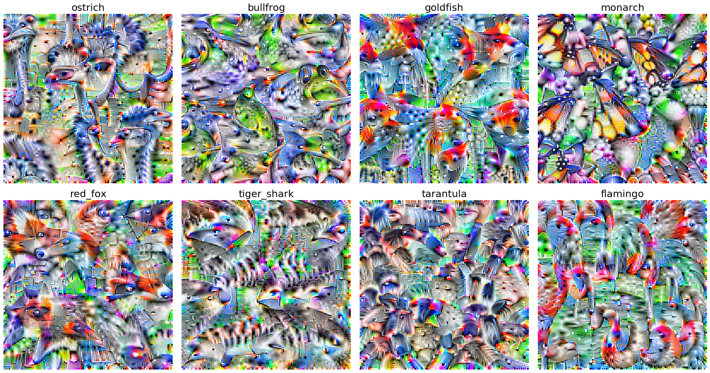
Fig. 34 Synthesized images that maximally activate class labels. The results are an artifact of using convolutions. Source#
import random
import warnings
from pathlib import Path

import numpy as np
import pandas as pd
import matplotlib.pyplot as plt
import matplotlib
from matplotlib_inline import backend_inline

import torch
import torch.nn as nn
import torch.nn.functional as F

DATASET_DIR = Path("./data/").resolve()
DATASET_DIR.mkdir(exist_ok=True)
warnings.simplefilter(action="ignore")
backend_inline.set_matplotlib_formats("svg")
matplotlib.rcParams["image.interpolation"] = "nearest"

RANDOM_SEED = 0
random.seed(RANDOM_SEED)
np.random.seed(RANDOM_SEED)
torch.manual_seed(RANDOM_SEED)

print(torch.__version__)
print(torch.backends.mps.is_built())
DEVICE = torch.device("mps")
2.0.0
True
Convolution operation#
Suppose we want to classify cat images using a linear model. Flattening the image into a vector and feeding it into a fully-connected network is not the best approach. The resulting input vector would be too long resulting in a very large weight matrix. Moreover, it does not consider local spatial correlation of image pixels (Fig. 35) (e. g. shuffling the input pixels by the same permutation at the start results in an equivalent network). This motivates only mixing nearby pixels in a linear combination resulting in a very sparse banded weight matrix (Fig. 36).
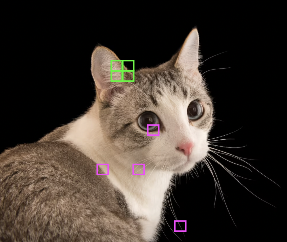
Fig. 35 Nearby pixels combine to form meaningful features of an image. Source#
Let \(\boldsymbol{\mathsf X}\) be an \(n \times n\) input image and \(\boldsymbol{\mathsf{S}}\) be the \(m \times m\) output feature map. The banded weight matrix reduces the nonzero entries of the weight matrix from \(m^2 n^2\) to \(m^2{k}^2\) where a local region of \(k \times k\) pixels in the input image are mixed. If the feature detector is translationally invariant across the image, then the weights in each band are shared. This further reduces the number of weights to \(k^2\)! The resulting linear operation is called a convolution in two spatial dimensions:
Observe that spatial ordering of the pixels in the input \(\boldsymbol{\mathsf X}\) is somewhat preserved in the output \(\boldsymbol{\mathsf{S}}.\) This is nice since we want spatial information and orientation across a stack of convolution operations to be preserved in the final output.
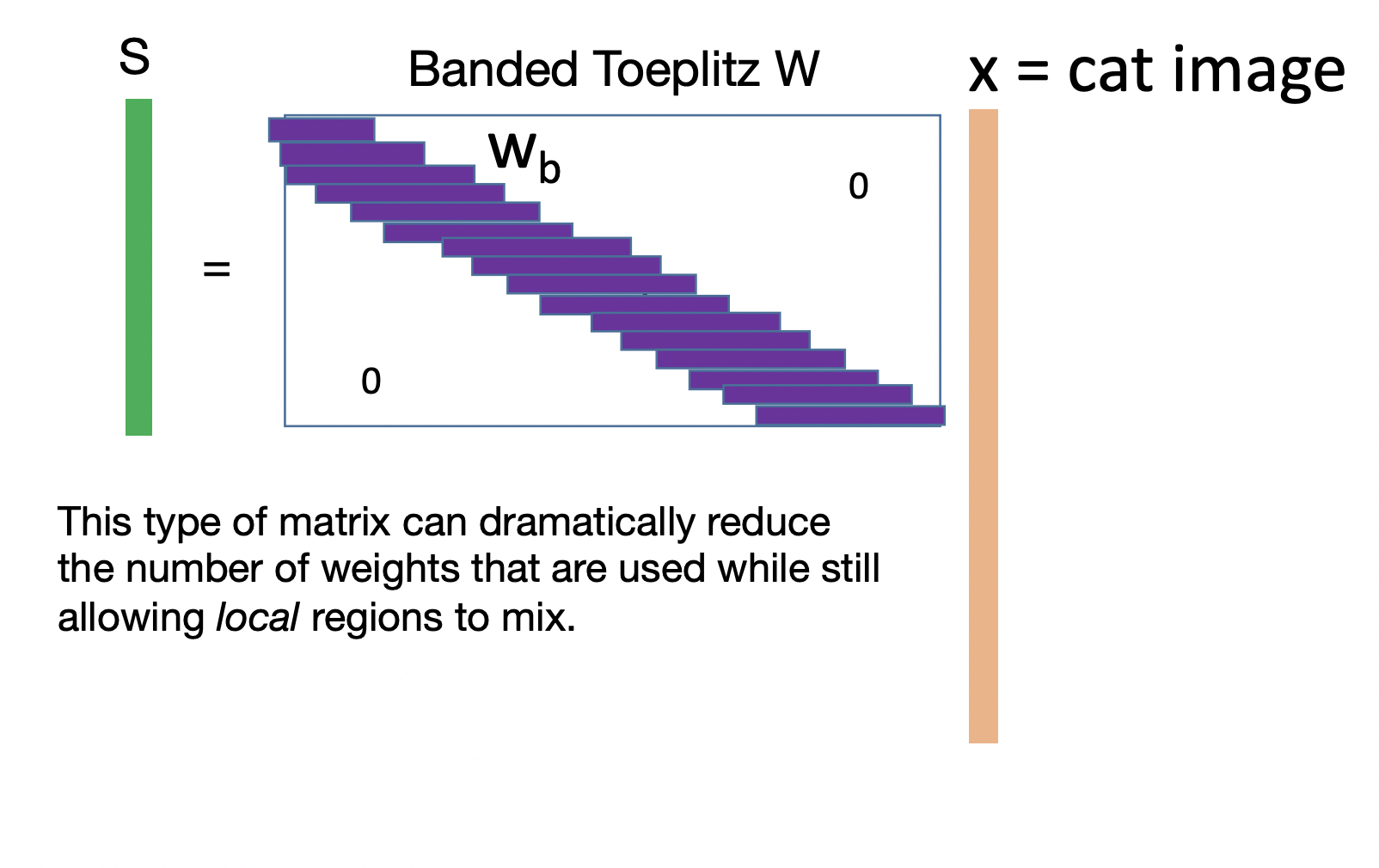
Fig. 36 Banded Toeplitz matrix for classifying cat images. The horizontal vectors contain the same pixel values. Note that there can be multiple bands for a 2D kernel. See this SO answer.#
Fig. 37 The following shows a convolution operation with 3 × 3 kernel for 2D input. This essentially visualizes (8). Source: vdumoulin/conv_arithmetic#
Convolution layer#
Recall that digital images have multiple channels. The convolution layer extends the convolution operation to handle feature maps with multiple channels. Similarly, the output feature map has channels as this adds a further semantic dimension to the downstream representation. For an RGB image, a convolution layer learns three 2-dimensional kernels \(\boldsymbol{\mathsf{K}}_{lc}\) for each output channel, each of which can be thought of as a feature extractor (like neurons in a dense layer). Note that features across input channels are blended by the kernel. This is expressed by the following formula:
for \(l = 0, \ldots, {c}_\text{out}-1\). The input and output tensors \(\boldsymbol{\mathsf{X}}\) and \(\bar{\boldsymbol{\mathsf{X}}}\) have the same dimensionality and semantic structure which makes sense since we want to stack convolutional layers as modules, and the kernel \(\boldsymbol{\mathsf{K}}\) has shape \(({c}_\text{out}, {c}_\text{in}, {k}, {k}).\) The resulting feature maps inherit the spatial ordering in its inputs along the spatial dimensions. Note that each convolution operation is independent for each output channel. Moreover, the entire operation is linear.
Remark. This is called 2D convolution since it processes inputs with 2 spatial dimensions indexed by \(i\) and \(j\). Meanwhile, 1D convolutions used for processing sequential data has 1 dimension (e.g. for time).
Reproducing the convolution operation over input and output channels:
from torchvision.io import read_image
import torchvision.transforms.functional as fn

def convolve(X, K):
    """Perform 2D convolution over input."""
    h, w = K.shape
    H0, W0 = X.shape
    H1 = H0 - h + 1
    W1 = W0 - w + 1

    S = np.zeros(shape=(H1, W1))
    for i in range(H1):
        for j in range(W1):
            S[i, j] = (X[i:i+h, j:j+w] * K).sum()

    return torch.tensor(S)


@torch.no_grad()
def conv_components(X, K, u):
    cmaps = ["Reds", "Greens", "Blues"]
    cmaps_out = ["spring", "summer", "autumn", "winter"]
    c_in  = X.shape[1]
    c_out = K.shape[0]

    fig, ax = plt.subplots(c_in + 1, c_out + 1, figsize=(12, 12))

    # Input image
    ax[0, 0].imshow(X[0].permute(1, 2, 0))
    for c in range(c_in):
        ax[c+1, 0].set_title(f"X(c={c})")
        ax[c+1, 0].imshow(X[0, c, :, :], cmap=cmaps[c])

    # Iterate over kernel filters
    out_components = {}
    for k in range(c_out):
        for c in range(c_in):
            out_components[(c, k)] = convolve(X[0, c, :, :], K[k, c, :, :])
            ax[c+1, k+1].imshow(out_components[(c, k)].numpy())
            ax[c+1, k+1].set_title(f"X(c={c}) ⊛ K(c={c}, k={k})")

    # Sum convolutions over input channels, then add bias
    out_maps = []
    for k in range(c_out):
        out_maps.append(sum([out_components[(c, k)] for c in range(c_in)]) + u[k])
        ax[0, k+1].imshow(out_maps[k].numpy(), cmaps_out[k])
        ax[0, k+1].set_title(r"$\bar{\mathrm{X}}$" + f"(k={k})")

    fig.tight_layout()
    return out_maps


cat = DATASET_DIR / "shorty.png"
X = read_image(str(cat)).unsqueeze(0)[:, :3, :, :]
X = fn.resize(X, size=(128, 128)) / 255.
conv = nn.Conv2d(in_channels=3, out_channels=4, kernel_size=5)
K, u = conv.weight, conv.bias
components = conv_components(X, K, u);

Figure. Each kernel in entries i,j > 0 combines column-wise with the inputs to compute X(c=i) ⊛ K(c=i, k=j). The sum of these terms over c form the output map X̅(k=j) above.
This looks similar to dense layers, but with convolutions between 2-dim matrices instead of products between scalar nodes. This allows convolutional networks to perform combinatorial mixing of (hierarchical) features with depth.
Checking if consistent with Conv2d in PyTorch:
Show code cell source
S = torch.stack(components).unsqueeze(0)
P = conv(X)
cmaps_out = ["spring", "summer", "autumn", "winter"]

print("Input shape: ", X.shape)   # (B, c0, H0, W0)
print("Output shape:", S.shape)   # (B, c1, H1, W1)
print("Kernel shape:", K.shape)   # (c1, c0, h, w)
print("Bias shape:  ", u.shape)   # (c1,)

# Check if above formula agrees with PyTorch implementation
print("MAE (w/ pytorch) =", (S - P).abs().mean().item())

# Plotting the images obtained using the above formula
print("\nOutput components (from scratch):")
fig, ax = plt.subplots(1, 4)
fig.tight_layout()
for k in range(4):
    ax[k].imshow(S[0, k].detach().numpy(), cmaps_out[k])
Input shape:  torch.Size([1, 3, 128, 128])
Output shape: torch.Size([1, 4, 124, 124])
Kernel shape: torch.Size([4, 3, 5, 5])
Bias shape:   torch.Size([4])
MAE (w/ pytorch) = 2.5097616801085692e-08

Output components (from scratch):

Show code cell source
# Plotting the images obtained using pytorch conv
print("\nOutput components (from pytorch):")
fig, ax = plt.subplots(1, 4)
fig.tight_layout()
for k in range(4):
    ax[k].imshow(P[0, k].detach().numpy(), cmaps_out[k])
Output components (from pytorch):

Padding and stride#
Stride. The step size of the kernel can be controlled using the stride parameter. A large stride along with a large kernel size can be useful if objects are large relative to the dimension of the image. Note that stride significantly reduces computation by constant factor. Strided convolutions have been used as an alternative way to downsample an image (i.e. works better or just as well as conv + pooling) [SDBR14]. Notice that the spatial size decreases with stride:
conv = lambda s: nn.Conv2d(in_channels=3, out_channels=3, stride=s, kernel_size=3)
fig, ax = plt.subplots(1, 4, figsize=(8, 2))

ax[0].imshow(X[0].permute(1, 2, 0))
ax[1].imshow(conv(1)(X)[0, 0].detach().numpy()); ax[1].set_title("s=1")
ax[2].imshow(conv(2)(X)[0, 0].detach().numpy()); ax[2].set_title("s=2")
ax[3].imshow(conv(3)(X)[0, 0].detach().numpy()); ax[3].set_title("s=3")
fig.tight_layout();

Padding. Edge pixels of an input image are underrepresented since the kernel has to be kept within the input image. Moreover, information in the edges become lost as we stack more convolutional layers. One solution is to pad the boundaries. The simplest to implement is zero padding. Observe the weird effect on the boundaries:
pad  = nn.ZeroPad2d(padding=3)  # zero pad 3 pixels on every side
conv = nn.Conv2d(3, 1, kernel_size=3)
Show code cell source
fig, ax = plt.subplots(2, 2, figsize=(5, 5))
vmin = min(conv(X).min(), conv(pad(X)).min())
vmax = max(conv(X).max(), conv(pad(X)).max())
ax[1, 0].imshow(pad(X)[0].permute(1, 2, 0).detach(), vmin=vmin, vmax=vmax); ax[1, 0].set_title("Pad(X)")
ax[1, 1].imshow(conv(pad(X))[0, 0].detach(),         vmin=vmin, vmax=vmax); ax[1, 1].set_title("Conv(Pad(X))")
ax[0, 0].imshow(X[0].permute(1, 2, 0).detach(),      vmin=vmin, vmax=vmax); ax[0, 0].set_title("X")
ax[0, 1].imshow(conv(X)[0, 0].detach(),              vmin=vmin, vmax=vmax); ax[0, 1].set_title("Conv(X)")
fig.tight_layout();

Remark. Padding and stride determines the spatial dimensions of the output feature maps. An input of width \(w\) and equal padding \(p\), and kernel size \(k\) with stride \(s\) has an output of width \(\lfloor(w + 2p - k)/s + 1\rfloor\). In particular, we have to carefully choose stride and padding values so that the kernel can be placed evenly in the image so that no input pixel is dropped.
For \({s} = 1,\) kernel size should be odd so that it covers the entire input in a symmetric manner. A common choice is \(p = (k - 1)/2\) which results in same sized outputs (i.e. the so-called same convolution). For \({s} > 1,\) the best practice is to choose a kernel size and the smallest \(p\) such that \(s\) divides \(w + 2p - k\) so that the entire input image is symmetrically covered by the kernel.
Downsampling#
The receptive field of a unit consists of all units from earlier layers that influence its value during forward pass (Fig. 38). In particular, units for each class in the softmax layer should have a receptive field that includes the entire input. Otherwise, some parts of the input will not affect the prediction of the model for that class. One way to increase receptive field, and make the network more robust to noise, is by downsampling the output feature maps. Here we do it along the spatial dimensions.
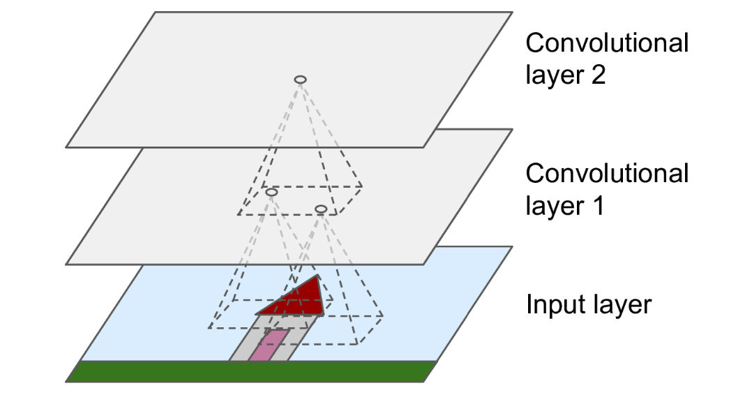
Fig. 38 Receptive field of a pixel in a convolutional network. For an output pixel in an intermediate layer, whose are inputs are formed from stacked convolutions, its larger receptive field indicates that it processes hierarchical features of the original image.#
Pooling layers. Pooling layers downsample an input by performing nonparametric operations and sliding across the input like convolutional layers. This can be interpreted as decreasing the resolution of feature maps (sort of zooming out) that deeper layers will work on. Pooling is applied to each channel separately, so that the number of output channels is maintained. This makes sense since we want only to compress the original input without affecting its semantic structure.
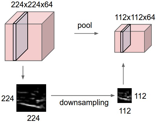
Fig. 39 Pooling layer downsamples the volume spatially independently in each channel. The input tensor of size 224 × 224 × 64 is pooled with filter size 2 and stride 2 into output volume of size 112 × 112 × 64.#
Max pooling. Max pooling layers make the network insensitive to noise or fine-grained details in the input at the cost of some information loss. It can be interpreted as a form of competition between neurons since the gradient only flows through the activated neuron. A soft alternative is average pooling. Commonly used parameters are k=2, s=2 where the pooling regions do not overlap, and k=3, s=2 where some overlap is allowed.
Show code cell source
x = torch.tensor([
    [ 1, 1, 2, 4],
    [ 4, 5, 6, 9],
    [ 3, 1, 0, 3],
    [ 4, 0, 1, 8]]
)[None, None, :, :].float()

pool = nn.MaxPool2d(kernel_size=2, stride=2)

# Plotting
fig, ax = plt.subplots(1, 2, figsize=(4, 2))
ax[0].set_title("X")
ax[0].imshow(x.numpy()[0, 0, :, :], cmap="viridis", vmin=0)
ax[0].set_xticks([])
ax[0].set_yticks([])
for i in range(4):
    for j in range(4):
        ax[0].text(j, i, int(x[0, 0, i, j].numpy()), ha="center", va="bottom", color="black")

ax[1].set_title("MaxPool(X)")
ax[1].imshow(pool(x)[0].detach().permute(1, 2, 0), cmap="viridis", vmin=0)
ax[1].set_xticks([])
ax[1].set_yticks([])
for i in range(2):
    for j in range(2):
        ax[1].text(j, i, int(pool(x)[0, 0, i, j].numpy()), ha="center", va="bottom", color="black")

fig.tight_layout()

Using a large kernel relative to the input can result in information loss:
Show code cell source
fig, ax = plt.subplots(1, 3, figsize=(8, 3))
ax[0].imshow(X[0, :, :, :].permute(1, 2, 0))
ax[0].set_title("Original")
ax[1].imshow(nn.MaxPool2d(kernel_size=2, stride=2)(X)[0, :, :, :].permute(1, 2, 0))
ax[1].set_title("k = 2, s = 2")
ax[2].imshow(nn.MaxPool2d(kernel_size=5, stride=3)(X)[0, :, :, :].permute(1, 2, 0))
ax[2].set_title("k = 5, s = 3");

Global pooling. Global pooling follows that intuition that we want to detect some patterns, but we do not care too much where exactly these patterns are (Fig. 40). A global average pooling (GAP) layer will also be used later for an image classification task allowing the network to learn one feature detector for each output channel.
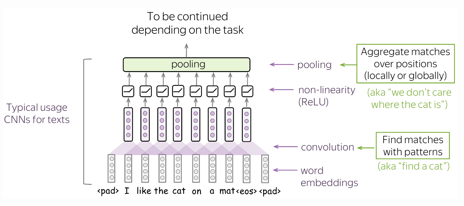
Fig. 40 A typical convolutional model for texts consist of conv + pooling blocks. Here convolutions are applicable when we want to classify text using the presence of local features (e.g. certain phrases). Source#
Training engine#
To separate concerns during model training, we define a trainer engine. For example, this defines an eval_context to automatically set the model to eval mode at entry, and back to the default train mode at exit. This is useful for layers such as BN and Dropout which have different behaviors at train and test times. LR schedulers and callbacks are also implemented. Currently, these are called at the end of each training step (it is easy to extend this class to implement epoch end callbacks).
from tqdm.notebook import tqdm
from contextlib import contextmanager
from torch.utils.data import DataLoader


@contextmanager
def eval_context(model):
    """Temporarily set to eval mode inside context."""
    state = model.training
    model.eval()
    try:
        yield
    finally:
        model.train(state)


class Trainer:
    def __init__(self,
        model, optim, loss_fn, scheduler=None, callbacks=[],
        device=DEVICE, verbose=True
    ):
        self.model = model.to(device)
        self.optim = optim
        self.device = device
        self.loss_fn = loss_fn
        self.train_log = {"loss": [], "accu": [], "loss_avg": [], "accu_avg": []}
        self.valid_log = {"loss": [], "accu": []}
        self.verbose = verbose
        self.scheduler = scheduler
        self.callbacks = callbacks

    def __call__(self, x):
        return self.model(x.to(self.device))

    def forward(self, batch):
        x, y = batch
        x = x.to(self.device)
        y = y.to(self.device)
        return self.model(x), y

    def train_step(self, batch):
        preds, y = self.forward(batch)
        accu = (preds.argmax(dim=1) == y).float().mean()
        loss = self.loss_fn(preds, y)
        loss.backward()
        self.optim.step()
        self.optim.zero_grad()
        return {"loss": loss, "accu": accu}

    @torch.inference_mode()
    def valid_step(self, batch):
        preds, y = self.forward(batch)
        accu = (preds.argmax(dim=1) == y).float().sum()
        loss = self.loss_fn(preds, y, reduction="sum")
        return {"loss": loss, "accu": accu}

    def run(self, epochs, train_loader, valid_loader, window_size=None):
        for e in tqdm(range(epochs)):
            for i, batch in enumerate(train_loader):
                # optim and lr step
                output = self.train_step(batch)
                if self.scheduler:
                    self.scheduler.step()

                # step callbacks
                for callback in self.callbacks:
                    callback()

                # logs @ train step
                steps_per_epoch = len(train_loader)
                w = int(0.05 * steps_per_epoch) if not window_size else window_size
                self.train_log["loss"].append(output["loss"].item())
                self.train_log["accu"].append(output["accu"].item())
                self.train_log["loss_avg"].append(np.mean(self.train_log["loss"][-w:]))
                self.train_log["accu_avg"].append(np.mean(self.train_log["accu"][-w:]))

            # logs @ epoch
            output = self.evaluate(valid_loader)
            self.valid_log["loss"].append(output["loss"])
            self.valid_log["accu"].append(output["accu"])
            if self.verbose:
                print(f"[Epoch: {e+1:>0{int(len(str(epochs)))}d}/{epochs}]    loss: {self.train_log['loss_avg'][-1]:.4f}  acc: {self.train_log['accu_avg'][-1]:.4f}    val_loss: {self.valid_log['loss'][-1]:.4f}  val_acc: {self.valid_log['accu'][-1]:.4f}")

    def evaluate(self, data_loader):
        with eval_context(self.model):
            valid_loss = 0.0
            valid_accu = 0.0
            for batch in data_loader:
                output = self.valid_step(batch)
                valid_loss += output["loss"].item()
                valid_accu += output["accu"].item()

        return {
            "loss": valid_loss / len(data_loader.dataset),
            "accu": valid_accu / len(data_loader.dataset)
        }

    @torch.inference_mode()
    def predict(self, x: torch.Tensor):
        with eval_context(self.model):
            return self(x)

    @torch.inference_mode()
    def batch_predict(self, input_loader: DataLoader):
        with eval_context(self.model):
            preds = [self(x) for x in input_loader]
            preds = torch.cat(preds, dim=0)
        return preds
The predict method is suited for inference over one transformed mini-batch. A model call over a large input tensor may cause memory error. The model does not generate a computational graph to conserve memory and calls the model with layers in eval mode. For large batches, one should use batch_predict which is the same but takes in a data loader with transforms.
model = nn.Sequential(nn.Linear(3, 10), nn.Dropout(1.0))
trainer = Trainer(model, optim=None, scheduler=None, loss_fn=None)

# inference mode using eval_context
x = torch.ones(size=(1, 3), requires_grad=True)
print(f"__call__    {(trainer(x) > 0).float().mean():.3f}")
print(f"predict     {(trainer.predict(x) > 0).float().mean():.3f}")
__call__    0.000
predict     0.400
Checking computational graph generation:
y = trainer(x)
z = trainer.predict(x)
print("__call__   ", y.requires_grad)
print("predict    ", z.requires_grad)
__call__    True
predict     False
Convolutional networks#
In this section, we implement LeNet-5 [LBBH98] and train it to classify handwritten digits in MNIST. In fact, this network was introduced in the 1990s to identify handwritten zip code numbers provided by the US Postal Service (Fig. 43). LeNet is characterized as having convolution and pooling blocks as feature extractor. Finally, the features are passed to an MLP with 10 final nodes corresponding to each class label.

Remark. A block is composed of multiple layers that together form a basic functional unit. This is generally used in designing neural net architectures. See also AlexNet [KSH12] and VGG [SZ14] which takes this network design to the extreme (Fig. 42). These networks also contain consecutive convolutional blocks that downsample the spatial dimensions, while increasing the number of output channels so that network capacity is not diminished.
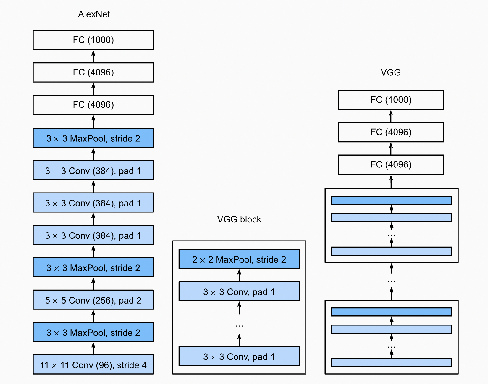
Fig. 42 Network architecture of AlexNet and VGG. More layers means more processing, which is why we see repeated convolutions and blocks. Source#
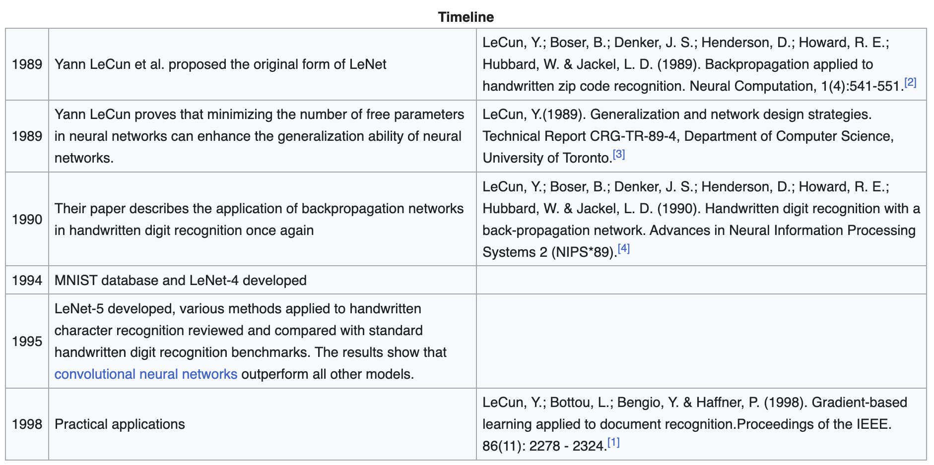
Fig. 43 A bit of history. Timeline of the development of LeNet and MNIST. Source#
Model#
import torchsummary

mnist_model = lambda: nn.Sequential(
    nn.Conv2d(1, 32, kernel_size=3, padding=1),
    nn.SELU(),
    nn.MaxPool2d(kernel_size=2, stride=2),

    nn.Conv2d(32, 32, kernel_size=5, padding=0),
    nn.SELU(),
    nn.MaxPool2d(kernel_size=2, stride=2),

    nn.Flatten(),
    nn.Linear(32 * 5 * 5, 256),
    nn.SELU(),
    nn.Dropout(0.5),
    nn.Linear(256, 10)
)

torchsummary.summary(mnist_model(), (1, 28, 28))
----------------------------------------------------------------
        Layer (type)               Output Shape         Param #
================================================================
            Conv2d-1           [-1, 32, 28, 28]             320
              SELU-2           [-1, 32, 28, 28]               0
         MaxPool2d-3           [-1, 32, 14, 14]               0
            Conv2d-4           [-1, 32, 10, 10]          25,632
              SELU-5           [-1, 32, 10, 10]               0
         MaxPool2d-6             [-1, 32, 5, 5]               0
           Flatten-7                  [-1, 800]               0
            Linear-8                  [-1, 256]         205,056
              SELU-9                  [-1, 256]               0
          Dropout-10                  [-1, 256]               0
           Linear-11                   [-1, 10]           2,570
================================================================
Total params: 233,578
Trainable params: 233,578
Non-trainable params: 0
----------------------------------------------------------------
Input size (MB): 0.00
Forward/backward pass size (MB): 0.50
Params size (MB): 0.89
Estimated Total Size (MB): 1.39
----------------------------------------------------------------
Remark. We use SELU activation [KUMH17] for fun. Note that we also used Dropout [SHK+14] as regularization for the dense layers. These will be discussed in a future notebook in this series. Observe that convolutions have small contribution to the total number of parameters of the network!
Setting up MNIST data loaders:
from torchvision import transforms
from torchvision.datasets import MNIST
from torch.utils.data import random_split, DataLoader

transform = transforms.Compose([
    transforms.ToTensor(),
    transforms.Lambda(lambda x: x / 255.)
])

mnist_all = MNIST(root=DATASET_DIR, download=True, transform=transform)
mnist_train, mnist_valid = random_split(
    mnist_all, [55000, 5000],
    generator=torch.Generator().manual_seed(RANDOM_SEED)
)

mnist_train_loader = DataLoader(mnist_train, batch_size=32, shuffle=True) # (!)
mnist_valid_loader = DataLoader(mnist_valid, batch_size=32, shuffle=False)
Remark. shuffle=True is important for SGD training. The model has low validation score when looping through the samples in the same order during training. This may be due to cyclic behavior in the updates (i.e. they cancel out).
LR scheduling#
Training the model with one-cycle LR schedule [ST17]. The one-cycle policy anneals the learning rate from an initial learning rate to some maximum learning rate and then from that maximum learning rate to some minimum learning rate much lower than the initial learning rate. Momentum is also annealed inversely to the learning rate which is necessary for stability.
from torch.optim.lr_scheduler import OneCycleLR

class SchedulerStatsCallback:
    def __init__(self, optim):
        self.lr = []
        self.momentum = []
        self.optim = optim

    def __call__(self):
        self.lr.append(self.optim.param_groups[0]["lr"])
        self.momentum.append(self.optim.param_groups[0]["betas"][0])

epochs = 3
model = mnist_model().to(DEVICE)
loss_fn = F.cross_entropy
optim = torch.optim.AdamW(model.parameters(), lr=0.001)
scheduler = OneCycleLR(optim, max_lr=0.01, steps_per_epoch=len(mnist_train_loader), epochs=epochs)
scheduler_stats = SchedulerStatsCallback(optim)
trainer = Trainer(model, optim, loss_fn, scheduler, callbacks=[scheduler_stats])
trainer.run(epochs=epochs, train_loader=mnist_train_loader, valid_loader=mnist_valid_loader)
[Epoch: 1/3]    loss: 1.5254  acc: 0.8734    val_loss: 0.9166  val_acc: 0.9360
[Epoch: 2/3]    loss: 0.3728  acc: 0.9491    val_loss: 0.2036  val_acc: 0.9660
[Epoch: 3/3]    loss: 0.1222  acc: 0.9717    val_loss: 0.0927  val_acc: 0.9798
Remark. After trying out other activations… SELU performance is surprising. It also trains really fast. That self-normalizing bit is no joke.
Show code cell source
from matplotlib.ticker import StrMethodFormatter

plt.figure(figsize=(8, 3))
plt.gca().yaxis.set_major_formatter(StrMethodFormatter("{x:,.2f}")) # 2 decimal places
plt.plot(np.array(trainer.train_log["accu"]), alpha=0.6, color="C1")
plt.plot(np.array(trainer.train_log["accu_avg"]), color="C1", label="train acc")
plt.plot(np.array(trainer.train_log["loss"]) / 10, alpha=0.6, color="C0")
plt.plot(np.array(trainer.train_log["loss_avg"]) / 10, color="C0", label="train loss")
plt.grid(linestyle="dotted")
plt.ylim(0.00, 1.05)
plt.legend();

plt.figure(figsize=(8, 1))
plt.plot(scheduler_stats.lr, color="black", label="lr")
plt.grid(linestyle="dotted")
plt.legend();

plt.figure(figsize=(8, 1))
plt.xlabel("step")
plt.plot(scheduler_stats.momentum, color="black", label=r"$\beta_1$")
plt.grid(linestyle="dotted")
plt.legend();


Figure. Note peak in train loss as LR increases to max_lr set at initialization, and the decreasing noise as the LR decreases at the end of training.
This works similarly with the LR finder which is a parameter-free method
described in a previous notebook for finding a good value for the base learning rate lr.
The bump in learning rate occurs over a wide duration during training,
so that the optimizer avoids many sharp minima.
This allows the network to train with less epochs — increasing the number of
epochs increases the exploration time (not just convergence time).
Feature maps#
Showing intermediate activations. Recall that feature map in the input of a convolutional layer is used to create each output feature map. Max-pooling and SELU on the other hand acts on each feature map independently. Note that fully-connected layer outputs are reshaped to two dimensions for the sake of presentation.
Show code cell source
from matplotlib.colors import LinearSegmentedColormap

x, y = next(iter(mnist_valid_loader))
b = torch.argmax((y == 8).type(torch.int64))
x = x[b:b+1, :].to(DEVICE) # first element

width_ratios = [1, 0.2, 1, 1, 1, 0.2, 1, 1, 1, 0.2, 0.6, 0.6, 0.6, 0.6, 0.8]
fig = plt.figure(figsize=(12, 5), constrained_layout=True)
spec = fig.add_gridspec(5, len(width_ratios), width_ratios=width_ratios)
cmap = LinearSegmentedColormap.from_list("custom", ["red", "white", "blue"])

# Input image
input_layer = []
for i in range(5):
    input_layer.append(fig.add_subplot(spec[i, 0]))
    input_layer[i].set_axis_off()

input_layer[2].imshow(x[0, 0].cpu().detach().numpy(), cmap="Greys")
input_layer[0].set_title("Input")

# Block 1
for k in range(3):
    x = model[k](x)
    layer = []
    for i in range(5):
        layer.append(fig.add_subplot(spec[i, k + 2]))
        layer[i].set_axis_off()
        layer[i].imshow(x[0, i+10].cpu().detach().numpy(), cmap="Greys")
        layer[i].axis("off")
    layer[0].set_title(type(model[k]).__name__)

# Block 2
for k in range(3):
    x = model[3 + k](x)
    layer = []
    for i in range(5):
        layer.append(fig.add_subplot(spec[i, k + 6]))
        layer[i].set_axis_off()
        layer[i].imshow(x[0, i].cpu().detach().numpy())
        layer[i].axis("off")
    layer[0].set_title(type(model[k]).__name__)

# Classification subnetwork
for l in range(5):
    x = model[6 + l](x)
    if l == 0:
        data = x[0].cpu().detach().view(-1, 8).numpy()
    elif l < 4:
        data = x[0].cpu().detach().view(-1, 4).numpy()
    else:
        data = x[0].cpu().detach().view(-1, 1).numpy()

    a = np.abs(data).max()
    ax = fig.add_subplot(spec[:, 10 + l])
    ax.imshow(data, cmap=cmap, vmin=-a, vmax=a)
    ax.xaxis.set_visible(False)
    ax.set_title(type(model[6 + l]).__name__)
    ax.tick_params(axis="y", colors="white")


# For last layer annotate value
for i in range(10):
    ax.tick_params(axis="y", colors="black")
    ax.set_yticks(range(10))
    ax.text(0, i, f"{data[i, 0]:.1f}", ha="center", va="center", color="black")

fig.tight_layout(pad=0.00)

Model predict probability (increase temperature to make the distribution look more random):
temp = 5.0
plt.figure(figsize=(4, 3))
plt.bar(range(10), F.softmax(x / temp, dim=1).detach().cpu()[0])
plt.xlabel("class")
plt.ylabel("predict proba.");

Data augmentation#
MNIST is not representative of real-world datasets. Below we continue with the Histopathologic Cancer Detection dataset from Kaggle where the task is to detect metastatic cancer in patches of images from digital pathology scans. Download the dataset such that the folder structure looks as follows:
!tree -L 1 ./data/histopathologic-cancer-detection
./data/histopathologic-cancer-detection
├── test
├── train
└── train_labels.csv

3 directories, 1 file
Taking a look at the first few images:
import cv2

IMG_DATASET_DIR = DATASET_DIR / "histopathologic-cancer-detection"
data = pd.read_csv(IMG_DATASET_DIR / "train_labels.csv")
fig, ax = plt.subplots(3, 5, figsize=(6, 4.5))

for k in range(15):
    i, j = divmod(k, 5)
    fname = str(IMG_DATASET_DIR / "train" / f"{data.id[k]}.tif")
    ax[i, j].imshow(cv2.imread(fname))
    ax[i, j].set_title(data.label[k], size=10)
    ax[i, j].axis("off")

fig.tight_layout()

A positive label indicates that the center 32 × 32 region of a patch contains at least one pixel of tumor tissue. Tumor tissue in the outer region of the patch does not influence the label. This outer region is provided to enable fully-convolutional models that do not use zero-padding, to ensure consistent behavior when applied to a whole-slide image.
Stochastic transforms#
Data augmentation incorporates transformed or perturbed versions of the original images into the dataset. More precisely, each data point \((\boldsymbol{\mathsf{x}}, y)\) in a mini-batch is replaced by \((T(\boldsymbol{\mathsf{x}}), y)\) during training where \(T\) is a stochastic label preserving transformation. At inference, an input \(\boldsymbol{\mathsf{x}}\) is replaced by \(\mathbb{E}[T(\boldsymbol{\mathsf{x}})].\)
transform_train = transforms.Compose([
    transforms.ToTensor(),
    transforms.RandomHorizontalFlip(),
    transforms.RandomVerticalFlip(),
    transforms.RandomRotation(20),
    transforms.CenterCrop([49, 49]),
])

transform_infer = transforms.Compose([
    transforms.ToTensor(),
    transforms.CenterCrop([49, 49]),
])
Recall that only the central pixels contribute to the labels. This motivates using center crop. Furthermore, we know that tissue samples in the slides can be flipped horizontally and vertically, as well as rotated (set to \(\pm 20^{\circ}\) above) without affecting the actual presence of tumor tissue.
from torch.utils.data import DataLoader, Dataset, Subset

class HistopathologicDataset(Dataset):
    def __init__(self, data, train=True, transform=None):
        split = "train" if train else "test"
        self.fnames = [str(IMG_DATASET_DIR / split / f"{fn}.tif") for fn in data.id]
        self.labels = data.label.tolist()
        self.transform = transform

    def __len__(self):
        return len(self.fnames)

    def __getitem__(self, index):
        img = cv2.imread(self.fnames[index])
        if self.transform:
            img = self.transform(img)

        return img, self.labels[index]


data = data.sample(frac=1.0)
split = int(0.80 * len(data))
histo_train_dataset = HistopathologicDataset(data[:split], train=True, transform=transform_train)
histo_valid_dataset = HistopathologicDataset(data[split:], train=True, transform=transform_infer)
Some imbalance (not too severe):
# percentage of positive class
data[:split].label.mean(), data[split:].label.mean()
(0.4050562436086808, 0.4049312578116123)
Simulating images across epochs:
simul_train = DataLoader(Subset(histo_train_dataset, torch.arange(3)), batch_size=3, shuffle=True)
simul_valid = DataLoader(Subset(histo_valid_dataset, torch.arange(1)), batch_size=1, shuffle=False)
Show code cell source
fig, ax = plt.subplots(3, 4)
for e in range(3):
    img_train, tgt_train = next(iter(simul_train))
    for i in range(3):
        if i == 0:
            ax[e, i].set_ylabel(f"Epoch:\n{e}")

        img, tgt = img_train[i], tgt_train[i]
        ax[e, i].imshow(img.permute(1, 2, 0).detach())
        ax[e, i].set_xlabel(tgt.item())
        ax[e, i].set_xticks([])
        ax[e, i].set_yticks([])
        ax[0, i].set_title(f"instance: {i}")

    img_valid, tgt_valid = next(iter(simul_valid))
    ax[e, 3].set_xlabel(tgt_valid[0].item())
    ax[e, 3].imshow(img_valid[0].permute(1, 2, 0).detach())
    ax[e, 3].set_xticks([])
    ax[e, 3].set_yticks([])

ax[0, 3].set_title("valid")
fig.tight_layout()

Figure. Inputs are stochastically transformed at each epoch. Note that the labels are not affected (both at the recognition and implementation level). The test and validation sets have fixed transformations implementing the expectation of the random transformations.
Transfer learning#
Transfer learning is a common technique for leveraging large models trained on related tasks (i.e. the so-called pretrained model). Here we will use ResNet [HZRS15a] trained on ImageNet which consists of millions of images in 1000 object categories. This requires us to replace the classification head which is task specific, and retain the feature extractors.
To not destroy the pretrained weights, we first train the classification head to convergence while keeping the weights of the pretrained model fixed. Then, we will proceed to fine-tune the pretrained weights with a low learning rate, again so that the pretrained weights are gradually changed.
import torchinfo
from torchvision import models

resnet = models.resnet18(pretrained=True)

BATCH_SIZE = 16
torchinfo.summary(resnet, input_size=(BATCH_SIZE, 3, 49, 49))
Show code cell output
==========================================================================================
Layer (type:depth-idx)                   Output Shape              Param #
==========================================================================================
ResNet                                   [16, 1000]                --
├─Conv2d: 1-1                            [16, 64, 25, 25]          9,408
├─BatchNorm2d: 1-2                       [16, 64, 25, 25]          128
├─ReLU: 1-3                              [16, 64, 25, 25]          --
├─MaxPool2d: 1-4                         [16, 64, 13, 13]          --
├─Sequential: 1-5                        [16, 64, 13, 13]          --
│    └─BasicBlock: 2-1                   [16, 64, 13, 13]          --
│    │    └─Conv2d: 3-1                  [16, 64, 13, 13]          36,864
│    │    └─BatchNorm2d: 3-2             [16, 64, 13, 13]          128
│    │    └─ReLU: 3-3                    [16, 64, 13, 13]          --
│    │    └─Conv2d: 3-4                  [16, 64, 13, 13]          36,864
│    │    └─BatchNorm2d: 3-5             [16, 64, 13, 13]          128
│    │    └─ReLU: 3-6                    [16, 64, 13, 13]          --
│    └─BasicBlock: 2-2                   [16, 64, 13, 13]          --
│    │    └─Conv2d: 3-7                  [16, 64, 13, 13]          36,864
│    │    └─BatchNorm2d: 3-8             [16, 64, 13, 13]          128
│    │    └─ReLU: 3-9                    [16, 64, 13, 13]          --
│    │    └─Conv2d: 3-10                 [16, 64, 13, 13]          36,864
│    │    └─BatchNorm2d: 3-11            [16, 64, 13, 13]          128
│    │    └─ReLU: 3-12                   [16, 64, 13, 13]          --
├─Sequential: 1-6                        [16, 128, 7, 7]           --
│    └─BasicBlock: 2-3                   [16, 128, 7, 7]           --
│    │    └─Conv2d: 3-13                 [16, 128, 7, 7]           73,728
│    │    └─BatchNorm2d: 3-14            [16, 128, 7, 7]           256
│    │    └─ReLU: 3-15                   [16, 128, 7, 7]           --
│    │    └─Conv2d: 3-16                 [16, 128, 7, 7]           147,456
│    │    └─BatchNorm2d: 3-17            [16, 128, 7, 7]           256
│    │    └─Sequential: 3-18             [16, 128, 7, 7]           8,448
│    │    └─ReLU: 3-19                   [16, 128, 7, 7]           --
│    └─BasicBlock: 2-4                   [16, 128, 7, 7]           --
│    │    └─Conv2d: 3-20                 [16, 128, 7, 7]           147,456
│    │    └─BatchNorm2d: 3-21            [16, 128, 7, 7]           256
│    │    └─ReLU: 3-22                   [16, 128, 7, 7]           --
│    │    └─Conv2d: 3-23                 [16, 128, 7, 7]           147,456
│    │    └─BatchNorm2d: 3-24            [16, 128, 7, 7]           256
│    │    └─ReLU: 3-25                   [16, 128, 7, 7]           --
├─Sequential: 1-7                        [16, 256, 4, 4]           --
│    └─BasicBlock: 2-5                   [16, 256, 4, 4]           --
│    │    └─Conv2d: 3-26                 [16, 256, 4, 4]           294,912
│    │    └─BatchNorm2d: 3-27            [16, 256, 4, 4]           512
│    │    └─ReLU: 3-28                   [16, 256, 4, 4]           --
│    │    └─Conv2d: 3-29                 [16, 256, 4, 4]           589,824
│    │    └─BatchNorm2d: 3-30            [16, 256, 4, 4]           512
│    │    └─Sequential: 3-31             [16, 256, 4, 4]           33,280
│    │    └─ReLU: 3-32                   [16, 256, 4, 4]           --
│    └─BasicBlock: 2-6                   [16, 256, 4, 4]           --
│    │    └─Conv2d: 3-33                 [16, 256, 4, 4]           589,824
│    │    └─BatchNorm2d: 3-34            [16, 256, 4, 4]           512
│    │    └─ReLU: 3-35                   [16, 256, 4, 4]           --
│    │    └─Conv2d: 3-36                 [16, 256, 4, 4]           589,824
│    │    └─BatchNorm2d: 3-37            [16, 256, 4, 4]           512
│    │    └─ReLU: 3-38                   [16, 256, 4, 4]           --
├─Sequential: 1-8                        [16, 512, 2, 2]           --
│    └─BasicBlock: 2-7                   [16, 512, 2, 2]           --
│    │    └─Conv2d: 3-39                 [16, 512, 2, 2]           1,179,648
│    │    └─BatchNorm2d: 3-40            [16, 512, 2, 2]           1,024
│    │    └─ReLU: 3-41                   [16, 512, 2, 2]           --
│    │    └─Conv2d: 3-42                 [16, 512, 2, 2]           2,359,296
│    │    └─BatchNorm2d: 3-43            [16, 512, 2, 2]           1,024
│    │    └─Sequential: 3-44             [16, 512, 2, 2]           132,096
│    │    └─ReLU: 3-45                   [16, 512, 2, 2]           --
│    └─BasicBlock: 2-8                   [16, 512, 2, 2]           --
│    │    └─Conv2d: 3-46                 [16, 512, 2, 2]           2,359,296
│    │    └─BatchNorm2d: 3-47            [16, 512, 2, 2]           1,024
│    │    └─ReLU: 3-48                   [16, 512, 2, 2]           --
│    │    └─Conv2d: 3-49                 [16, 512, 2, 2]           2,359,296
│    │    └─BatchNorm2d: 3-50            [16, 512, 2, 2]           1,024
│    │    └─ReLU: 3-51                   [16, 512, 2, 2]           --
├─AdaptiveAvgPool2d: 1-9                 [16, 512, 1, 1]           --
├─Linear: 1-10                           [16, 1000]                513,000
==========================================================================================
Total params: 11,689,512
Trainable params: 11,689,512
Non-trainable params: 0
Total mult-adds (G): 1.99
==========================================================================================
Input size (MB): 0.46
Forward/backward pass size (MB): 37.34
Params size (MB): 46.76
Estimated Total Size (MB): 84.56
==========================================================================================
in_features = resnet.fc.in_features
num_hidden = 256

head = nn.Sequential(
    nn.AdaptiveAvgPool2d(1),
    nn.Flatten(),
    nn.BatchNorm1d(in_features),
    nn.Dropout(0.5),
    nn.Linear(in_features, num_hidden),
    nn.ReLU(),
    nn.BatchNorm1d(num_hidden),
    nn.Dropout(0.5),
    nn.Linear(num_hidden, 2),
)

model = nn.Sequential(
    nn.Sequential(*list(resnet.children())[:-2]),
    head
)
Remark. This network is fairly deep, so we use batch normalization (BN) [IS15] to aid with activation and gradient stability. BN is discussed in more detail in a future notebook. Dropout is also used to regularize the dense layers.
Static features#
Freezing the feature extraction layers:
for param in model[0].parameters(): # model[0] = pretrained
    param.requires_grad = False
Setting up the data loaders:
histo_train_loader = DataLoader(Subset(histo_train_dataset, torch.arange(32000)), batch_size=BATCH_SIZE, shuffle=True)
histo_valid_loader = DataLoader(Subset(histo_valid_dataset, torch.arange(8000)),  batch_size=BATCH_SIZE, shuffle=False)
Training the model using AdamW [LH17] with learning rate 0.001:
epochs = 10
optim = torch.optim.AdamW(model.parameters(), lr=0.001)
scheduler = OneCycleLR(optim, max_lr=0.01, steps_per_epoch=len(histo_train_loader), epochs=epochs)
trainer = Trainer(model, optim, loss_fn=F.cross_entropy, scheduler=scheduler, device=DEVICE)
trainer.run(epochs=epochs, train_loader=histo_train_loader, valid_loader=histo_valid_loader)
[Epoch: 01/10]    loss: 0.6182  acc: 0.6725    val_loss: 0.5455  val_acc: 0.7491
[Epoch: 02/10]    loss: 0.5777  acc: 0.6944    val_loss: 0.5170  val_acc: 0.7536
[Epoch: 03/10]    loss: 0.5864  acc: 0.6994    val_loss: 0.5243  val_acc: 0.7450
[Epoch: 04/10]    loss: 0.5556  acc: 0.7231    val_loss: 0.5036  val_acc: 0.7671
[Epoch: 05/10]    loss: 0.5817  acc: 0.7113    val_loss: 0.5229  val_acc: 0.7526
[Epoch: 06/10]    loss: 0.5689  acc: 0.7087    val_loss: 0.5081  val_acc: 0.7551
[Epoch: 07/10]    loss: 0.5523  acc: 0.7125    val_loss: 0.5007  val_acc: 0.7676
[Epoch: 08/10]    loss: 0.5657  acc: 0.7175    val_loss: 0.4882  val_acc: 0.7728
[Epoch: 09/10]    loss: 0.5301  acc: 0.7362    val_loss: 0.4823  val_acc: 0.7741
[Epoch: 10/10]    loss: 0.5332  acc: 0.7438    val_loss: 0.4805  val_acc: 0.7782
Show code cell content
def plot_training_history(trainer):
    fig, ax = plt.subplots(1, 2, figsize=(8, 4))
    num_epochs = len(trainer.valid_log["accu"])
    num_steps_per_epoch = len(trainer.train_log["accu"]) // num_epochs
    ax[0].plot(trainer.train_log["loss"], alpha=0.3, color="C0")
    ax[1].plot(trainer.train_log["accu"], alpha=0.3, color="C0")
    ax[0].plot(trainer.train_log["loss_avg"], label="train", color="C0")
    ax[1].plot(trainer.train_log["accu_avg"], label="train", color="C0")
    ax[0].plot(list(range(num_steps_per_epoch, (num_epochs + 1) * num_steps_per_epoch, num_steps_per_epoch)), trainer.valid_log["loss"], label="valid", color="C1")
    ax[1].plot(list(range(num_steps_per_epoch, (num_epochs + 1) * num_steps_per_epoch, num_steps_per_epoch)), trainer.valid_log["accu"], label="valid", color="C1")
    ax[0].set_xlabel("step")
    ax[0].set_ylabel("loss")
    ax[0].grid(linestyle="dashed", alpha=0.3)
    ax[1].set_xlabel("step")
    ax[1].set_ylabel("accuracy")
    ax[1].grid(linestyle="dashed", alpha=0.3)
    ax[1].legend()
    ax[0].set_ylim(0, max(trainer.train_log["loss"]))
    ax[1].set_ylim(0, 1)
    ax[0].ticklabel_format(axis="x", style="sci", scilimits=(3, 3))
    ax[1].ticklabel_format(axis="x", style="sci", scilimits=(3, 3))

    fig.tight_layout();
plot_training_history(trainer)

Remark. The validation step accumulates results over after an epoch for a fixed set of weights. This simulates inference performance if we load the trained model at that checkpoint. On the other hand, train metrics are expensive since the training dataset is large. Instead, these are accumulated at each step as an average with the previous steps.
Fine-tuning#
Unfreezing the pretrained model layers. Note that we set small learning rates:
for param in model[0].parameters():
    param.requires_grad = True

# 10X smaller lr (both optim and scheduler!)
epochs = 20
optim = torch.optim.AdamW(model.parameters(), lr=0.0001)
scheduler = OneCycleLR(optim, max_lr=0.001, steps_per_epoch=len(histo_train_loader), epochs=epochs)
trainer_ft = Trainer(model, optim, loss_fn=F.cross_entropy, scheduler=scheduler, device=DEVICE)
trainer_ft.run(epochs=epochs, train_loader=histo_train_loader, valid_loader=histo_valid_loader)
[Epoch: 01/20]    loss: 0.4119  acc: 0.8269    val_loss: 0.3713  val_acc: 0.8427
[Epoch: 02/20]    loss: 0.3827  acc: 0.8413    val_loss: 0.3606  val_acc: 0.8481
[Epoch: 03/20]    loss: 0.3982  acc: 0.8350    val_loss: 0.3591  val_acc: 0.8486
[Epoch: 04/20]    loss: 0.4048  acc: 0.8131    val_loss: 0.4162  val_acc: 0.8468
[Epoch: 05/20]    loss: 0.3909  acc: 0.8350    val_loss: 0.4206  val_acc: 0.8066
[Epoch: 06/20]    loss: 0.4052  acc: 0.8137    val_loss: 0.3880  val_acc: 0.8286
[Epoch: 07/20]    loss: 0.3636  acc: 0.8400    val_loss: 0.3679  val_acc: 0.8458
[Epoch: 08/20]    loss: 0.3587  acc: 0.8525    val_loss: 0.3551  val_acc: 0.8565
[Epoch: 09/20]    loss: 0.3830  acc: 0.8413    val_loss: 0.3992  val_acc: 0.8364
[Epoch: 10/20]    loss: 0.3504  acc: 0.8550    val_loss: 0.3462  val_acc: 0.8541
[Epoch: 11/20]    loss: 0.3266  acc: 0.8694    val_loss: 0.3417  val_acc: 0.8689
[Epoch: 12/20]    loss: 0.3608  acc: 0.8406    val_loss: 0.3500  val_acc: 0.8559
[Epoch: 13/20]    loss: 0.3287  acc: 0.8650    val_loss: 0.3992  val_acc: 0.8165
[Epoch: 14/20]    loss: 0.2955  acc: 0.8888    val_loss: 0.3053  val_acc: 0.8848
[Epoch: 15/20]    loss: 0.2975  acc: 0.8881    val_loss: 0.3336  val_acc: 0.8695
[Epoch: 16/20]    loss: 0.3060  acc: 0.8762    val_loss: 0.3147  val_acc: 0.8932
[Epoch: 17/20]    loss: 0.2738  acc: 0.8869    val_loss: 0.2823  val_acc: 0.8929
[Epoch: 18/20]    loss: 0.2424  acc: 0.9044    val_loss: 0.3039  val_acc: 0.8944
[Epoch: 19/20]    loss: 0.2889  acc: 0.8844    val_loss: 0.3175  val_acc: 0.8962
[Epoch: 20/20]    loss: 0.2986  acc: 0.8806    val_loss: 0.2892  val_acc: 0.8964
Show code cell source
loss = trainer.train_log["loss"] + trainer_ft.train_log["loss"]
accu = trainer.train_log["accu"] + trainer_ft.train_log["accu"]
loss_avg = trainer.train_log["loss_avg"] + trainer_ft.train_log["loss_avg"]
accu_avg = trainer.train_log["accu_avg"] + trainer_ft.train_log["accu_avg"]
val_loss = trainer.valid_log["loss"] + trainer_ft.valid_log["loss"]
val_accu = trainer.valid_log["accu"] + trainer_ft.valid_log["accu"]
num_epochs = len(val_loss)
num_steps_per_epoch = len(loss) // num_epochs

fig, ax = plt.subplots(1, 2, figsize=(8, 4))
ax[0].plot(loss, alpha=0.3, color="C0")
ax[1].plot(accu, alpha=0.3, color="C0")
ax[0].plot(loss_avg, label="train", color="C0")
ax[1].plot(accu_avg, label="train", color="C0")
ax[0].plot(list(range(num_steps_per_epoch, (num_epochs + 1) * num_steps_per_epoch, num_steps_per_epoch)), val_loss, label="valid", color="C1")
ax[1].plot(list(range(num_steps_per_epoch, (num_epochs + 1) * num_steps_per_epoch, num_steps_per_epoch)), val_accu, label="valid", color="C1")
ax[0].axvline(len(trainer.train_log["loss"]), color="black", linestyle="dotted", label="[fine-tuning]")
ax[1].axvline(len(trainer.train_log["loss"]), color="black", linestyle="dotted", label="[fine-tuning]")
ax[0].set_xlabel("step")
ax[0].set_ylabel("loss")
ax[0].grid(linestyle="dashed", alpha=0.3)
ax[0].set_ylim(0, max(loss))
ax[1].set_xlabel("step")
ax[1].set_ylabel("accuracy")
ax[1].grid(linestyle="dashed", alpha=0.3)
ax[1].set_ylim(0, 1)
ax[1].legend(framealpha=1.0)
ax[0].ticklabel_format(axis="x", style="sci", scilimits=(3, 3))
ax[1].ticklabel_format(axis="x", style="sci", scilimits=(3, 3))
fig.tight_layout();

Figure. First part trains the weights of the classification head steadily improving accuracy on the outputs of the frozen pretrained ResNet model. Then, we fine-tune the pretrained weights with a small learning rate resulting in substantial gains in accuracy.
Remarks. If we turn off data augmentation the validation curves diverge and the model overfits very early in the training (i.e. model memorizes the training data). Data augmentation prevents this by adding noise in the input. The dense layers also does not train well without BN. Recall that the data is imbalanced, so it is imperative to look at further evaluation tools such as the confusion matrix and PR curve.
Inference#
The trainer batch_predict method takes a data loader for inference. Note that simply calling the model on an input x may cause memory error for large models. Hence, using a data loader inference is good practice:
class InputDataLoader(DataLoader):
    def __init__(self, data_loader):
        self.data_loader = data_loader

    def __iter__(self):
        for batch in self.data_loader:
            yield batch[0]

pred = trainer.batch_predict(InputDataLoader(histo_valid_loader))
print(pred.shape)
print(pred)
torch.Size([8000, 2])
tensor([[-0.0891,  0.0826],
        [ 1.3988, -1.3978],
        [ 0.8117, -0.8179],
        ...,
        [ 0.6872, -0.6948],
        [-2.5100,  2.5002],
        [-1.9313,  1.9201]], device='mps:0')
This should be equal to the final validation accuracy:
y = torch.cat([batch[1] for batch in histo_valid_loader], dim=0)
print((pred.argmax(dim=1) == y.to(DEVICE)).float().mean().item())
print(trainer_ft.evaluate(histo_valid_loader)["accu"])
print(trainer_ft.valid_log["accu"][-1]) # or look at final valid log
0.8963750600814819
0.896375
0.896375
Remark. Recall that data points in our data loader come transformed. For processing raw images, we may have to call the eval mode transformation during model deployment as follows:
file_path = "data/histopathologic-cancer-detection/test/0a0a1f3867f41e02353afcaf503f63be1bdd35ec.tif"
test_data = cv2.imread(file_path)
print(trainer.predict(transform_infer(test_data).unsqueeze(0)))
tensor([[ 1.3396, -1.3394]], device='mps:0')
Appendix: Guided Backprop#
To explain the outputs of convolutional networks, we can look at the effect of each pixel in the input on each output node corresponding to a class. That is, we consider gradients \(\partial y / {\partial \boldsymbol{\mathsf{X}}^{\ell}}_{ij}\) for a target class \(y\) where \(\ell = 0\) for the input image. Note that gradients can be negative in intermediate layers, so to get a stronger signal we mask these gradients when computing backpropagation with respect to \({\boldsymbol{\mathsf{X}}^0}_{ij}\). In effect, we backpropagate only through those neurons which cause a first-order increase in the target class \(y\).
Moreover, positive activation indicate pattern detection for each node, hence we mask out nodes with negative activations further strengthening the signal. Since this is applied to all layers, we get patterns which are compositional and would eventually result in a positive activation for the target node. The gradients on input pixels are calculated with these two masks in place. This method is called Guided Backpropagation (GB) [SDBR14] used to obtain fine-grained details in the input image that contribute to the target class.
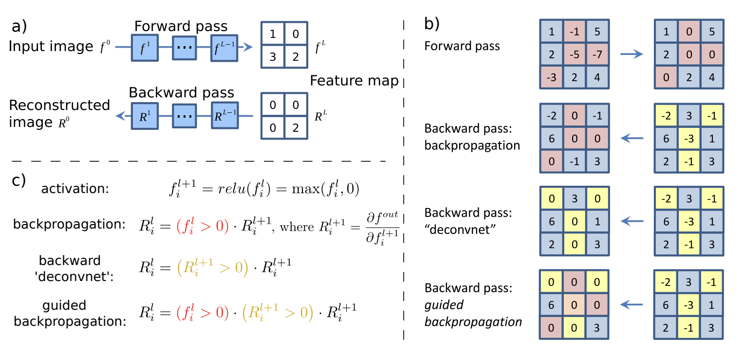
Fig. 44 Schematic of visualizing the activations of high layer neurons. Source: Fig. 1 of [SDBR14]#
def standardize_and_clip(x, min_val=0.0, max_val=1.0, saturation=0.1, brightness=0.5):
    x = x.detach().cpu()
    u = x.mean()
    v = max(x.std(), 1e-7)
    standardized = x.sub(u).div(v).mul(saturation)
    clipped = standardized.add(brightness).clamp(min_val, max_val)
    return clipped

def relu_hook_function(module, grad_in, grad_out):
    # Mask out negative gradients, and negative outputs
    # Note: ∂relu(x)/∂x = [x > 0] = [relu(x) > 0],
    # so that ∂(relu input) = [relu(x) > 0] * ∂(relu output).
    # This explains why we take the gradient wrt relu input.
    return (torch.clamp(grad_in[0], min=0.),)

def resize(x):
    return transforms.Resize(size=(224, 224))(x)

def register_hooks(model):
    hooks = []
    for _, module in model.named_modules():
        if isinstance(module, torch.nn.ReLU):
            h = module.register_backward_hook(relu_hook_function)
            hooks.append(h)
    return hooks

def guided_backprop(model, x, target=None):
    hooks = register_hooks(model)

    # backward through target node
    with eval_context(model):
        p = model(x)
        if target is None:
            target = p.argmax().item()

        y = p[0, target]
        y.backward()

    g = standardize_and_clip(x.grad)

    # cleanup (gradients and hooks)
    for _, module in model.named_modules():
        module.zero_grad()

    for h in hooks:
        h.remove()

    return {
        "x": resize(x[0]),
        "g": resize(g[0]).max(dim=0)[0],    # <- max guided backprop!, 1×H×W map.
        "p": F.softmax(p, dim=1)[0, target]
    }


# viz pathological tissue samples
outs = {}
target = 1
num_samples = 3
for b in range(num_samples):

    # prepare input image
    filepath = "data/histopathologic-cancer-detection/train"
    filename = data[data.label == target].iloc[b, 0]
    image = f"{filepath}/{filename}.tif"
    x = transform_infer(cv2.imread(image)).unsqueeze(0).to(DEVICE)
    x.requires_grad = True

    # magic happening...
    outs[b] = guided_backprop(model, x, target)
Remark. The backward hooks for masking negative gradients are only attached to ReLU layers since the network only has ReLU activations. See comments in the code. For other activations, you may need to implement forward hooks to mask out negative activations.
Note that backward hooks are executed before the tensor saves its gradients. Moreover, its return value modifies the input gradients of the given module. Finally, we take the maximum for each input image channel to get a grayscale map for the gradients.
def normalize(x):
    """Map pixels to [0, 1]."""
    return (x - x.min()) / (x.max() - x.min())

# these can be sliders in a viz. app
min_val = 0.5
max_val = 10.0
overlay_alpha = 0.75
Show code cell source
fig, ax = plt.subplots(num_samples, 3, figsize=(5, 6))
for b in range(num_samples):
    ax[b, 0].imshow(normalize(outs[b]["x"]).detach().permute(1, 2, 0).cpu().numpy())
    ax[b, 1].imshow(standardize_and_clip(outs[b]["g"], min_val=min_val, max_val=max_val).cpu().numpy(), cmap="viridis")
    ax[b, 2].imshow(normalize(outs[b]["x"]).detach().permute(1, 2, 0).cpu().numpy())
    ax[b, 2].imshow(standardize_and_clip(outs[b]["g"], min_val=min_val, max_val=max_val).cpu().numpy(), cmap="viridis", alpha=overlay_alpha)
    ax[b, 0].axis("off")
    ax[b, 1].axis("off")
    ax[b, 2].axis("off")
    ax[b, 0].set_title(f"p({target} | x) = {outs[b]['p']:.3f}", size=8)
    ax[b, 1].set_title("Guided Backprop", size=8)
    ax[b, 2].set_title("Overlay", size=8)

fig.tight_layout()

Not a domain expert on histopathology, so let us compare how this looks like with pretrained AlexNet on a dog image.
transform = transforms.Compose([
    transforms.ToTensor(),
    transforms.Resize(224),
    transforms.CenterCrop(224),
    transforms.Normalize([0.485, 0.456, 0.406], [0.229, 0.224, 0.225])
])

image = cv2.imread("./data/shorty.png")
x = transform(image).unsqueeze(0).to(DEVICE)
x.requires_grad = True

alexnet = models.alexnet(pretrained=True).to(DEVICE)
out = guided_backprop(alexnet, x, target=None)
Show code cell source
min_val = 0.5
max_val = 10.0
overlay_alpha = 0.75
fig, ax = plt.subplots(1, 3, figsize=(8, 10))
ax[0].imshow(normalize(out["x"]).detach().permute(1, 2, 0).cpu().numpy())
ax[1].imshow(standardize_and_clip(out["g"], min_val=min_val, max_val=max_val).cpu().numpy(), cmap="viridis")
ax[2].imshow(normalize(out["x"]).detach().permute(1, 2, 0).cpu().numpy())
ax[2].imshow(standardize_and_clip(out["g"], min_val=min_val, max_val=max_val).cpu().numpy(), cmap="viridis", alpha=overlay_alpha)
ax[0].axis("off")
ax[1].axis("off")
ax[2].axis("off")
ax[0].set_title(f"p = {out['p']:.3f}\n(1000 classes)", size=8)
ax[1].set_title("Guided Backprop", size=8)
ax[2].set_title("Overlay", size=8);

Remark. It’s interesting that the model can pick out the whiskers from the input image.
Appendix: Text classification#
In this section, we train a convolutional network on text embeddings. In particular, our dataset consist of Spanish given names downloaded from jvalhondo/spanish-names-surnames. Our task is to classify names into its gender label given in this dataset.
!wget -O ./data/spanish-male-names.csv https://raw.githubusercontent.com/jvalhondo/spanish-names-surnames/master/male_names.csv
!wget -O ./data/spanish-female-names.csv https://raw.githubusercontent.com/jvalhondo/spanish-names-surnames/master/female_names.csv
Show code cell output
--2024-02-21 06:19:30--  https://raw.githubusercontent.com/jvalhondo/spanish-names-surnames/master/male_names.csv
Resolving raw.githubusercontent.com (raw.githubusercontent.com)... 185.199.108.133, 185.199.110.133, 185.199.111.133, ...
Connecting to raw.githubusercontent.com (raw.githubusercontent.com)|185.199.108.133|:443... connected.
HTTP request sent, awaiting response... 200 OK
Length: 491187 (480K) [text/plain]
Saving to: ‘./data/spanish-male-names.csv’

./data/spanish-male 100%[===================>] 479.67K   600KB/s    in 0.8s

2024-02-21 06:19:32 (600 KB/s) - ‘./data/spanish-male-names.csv’ saved [491187/491187]

--2024-02-21 06:19:32--  https://raw.githubusercontent.com/jvalhondo/spanish-names-surnames/master/female_names.csv
Resolving raw.githubusercontent.com (raw.githubusercontent.com)... 185.199.110.133, 185.199.111.133, 185.199.109.133, ...
Connecting to raw.githubusercontent.com (raw.githubusercontent.com)|185.199.110.133|:443... connected.
HTTP request sent, awaiting response... 200 OK
Length: 493597 (482K) [text/plain]
Saving to: ‘./data/spanish-female-names.csv’

./data/spanish-fema 100%[===================>] 482.03K  1.86MB/s    in 0.3s

2024-02-21 06:19:33 (1.86 MB/s) - ‘./data/spanish-female-names.csv’ saved [493597/493597]
dfm = pd.read_csv(DATASET_DIR / "spanish-male-names.csv")
dff = pd.read_csv(DATASET_DIR / "spanish-female-names.csv")

dfm = dfm[["name"]].dropna(axis=0, how="any")
dff = dff[["name"]].dropna(axis=0, how="any")
dfm["gender"] = "M"
dff["gender"] = "F"

df = pd.concat([dfm, dff], axis=0)
df["name"] = df.name.map(lambda s: s.replace(" ", "_").lower())
df = df.drop_duplicates().reset_index()
df
| index | name | gender | |
|---|---|---|---|
| 0 | 0 | antonio | M |
| 1 | 1 | jose | M |
| 2 | 2 | manuel | M |
| 3 | 3 | francisco | M |
| 4 | 4 | juan | M |
| ... | ... | ... | ... |
| 49334 | 24751 | zhihui | F |
| 49335 | 24752 | zoila_esther | F |
| 49336 | 24753 | zsanett | F |
| 49337 | 24754 | zuleja | F |
| 49338 | 24755 | zulfiya | F |
49339 rows × 3 columns
df.gender.value_counts()
gender
F    24755
M    24584
Name: count, dtype: int64
Looking at name lengths. The following histogram is multimodal due to having multiple subnames separated by space.
Show code cell source
from collections import Counter

name_length = Counter([len(n) for n in df.name])
lengths = sorted(name_length.keys())
plt.figure(figsize=(5, 3))
plt.bar(lengths, [name_length[k] for k in lengths])
plt.xlabel("Name length")
plt.ylabel("Count")
print("Max name length:", max(lengths))
Max name length: 27

len(df[df.name.apply(len) < 23]) / len(df)
0.9997365167514543
We pad names with . at the end so that we get same length names, with long names truncated to a max length. This is typical for language models due to architectural constraints. In any case, considering a sufficiently large fixed number of initial characters of a name should be enough to determine the label.
MAX_LEN = 22
CHARS = ["."] + sorted(list(set([c for n in df.name for c in n])))
VOCAB_SIZE = len(CHARS)

print("token count:", VOCAB_SIZE)
print("".join(CHARS))
token count: 31
.'_abcdefghijklmnopqrstuvwxyzçñ
Data loaders#
from torch.utils.data import Dataset, DataLoader

class NamesDataset(Dataset):
    def __init__(self, names: list[str], label: list[int]):
        self.char_to_int = {c: i for i, c in enumerate(CHARS)}
        self.data = torch.tensor([self.encode(name) for name in names])
        self.label = torch.tensor(label)

    def encode(self, name: str):
        return [self.char_to_int[char] for char in self.preprocess(name)]

    def decode(self, x: torch.Tensor):
        int_to_char = {i: c for c, i in self.char_to_int.items()}
        return "".join(int_to_char[i.item()] for i in x)

    def __len__(self):
        return len(self.data)

    def __getitem__(self, idx):
        return self.data[idx], self.label[idx]

    @staticmethod
    def preprocess(name):
        out = [c for c in name if c in CHARS]
        return "." + "".join(out)[:min(len(out), MAX_LEN)] + "." * (MAX_LEN - len(out))


label_map = lambda t: 1 if t == "F" else 0
g = torch.Generator().manual_seed(RANDOM_SEED)
names = df.name.tolist()
label = list(map(label_map, df.gender.tolist()))

names_dataset = NamesDataset(names, label)
names_train_dataset, names_valid_dataset = random_split(names_dataset, [0.8, 0.2], generator=g)
names_train_loader = DataLoader(names_train_dataset, batch_size=32, shuffle=True)
names_valid_loader = DataLoader(names_valid_dataset, batch_size=32, shuffle=False)
Sample instance:
x, y = next(iter(names_train_loader))
x[0], y[0]
(tensor([ 0, 12, 17, 10, 16,  2,  3, 16,  6, 20,  7, 25,  0,  0,  0,  0,  0,  0,
          0,  0,  0,  0,  0]),
 tensor(0))
Decoding:
name = names_dataset.decode(x[0])
name, "F" if label_map(y[0].item()) == 1 else "M"
('.john_andrew...........', 'M')
Model#
For each token (i.e. character in CHARS) we learn an embedding vector in \(\mathbb{R}^{10}.\) The convolution kernel runs across a context of characters with stride 1. Subnames are short, so a context size of 3 or 4 should be good. This is implemented below with a 1D convolution with kernel size equal to context size times the embedding size, and a stride equal to the embedding size (Fig. 45).
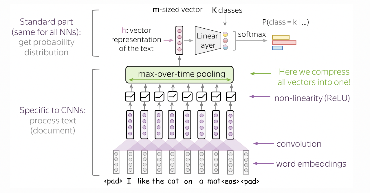
Fig. 45 Model architecture to classify text using convolutions. The kernel slides over embeddings instead of pixels. Source#
Hence, the model determines the gender label of a name by looking at the presence of certain n-grams in a name, regardless of its position in the name. This is done using max pool over time (Fig. 46) which reduces the feature map to a vector of length equal to the output channel of the 1D convolution.
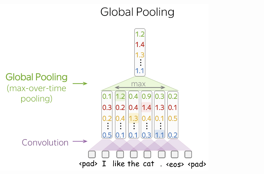
Fig. 46 Max pooling over time reduces the feature map to a vector whose entries correspond to the largest value in each output channel over the entire sequence. Source#
Note that we learn embeddings because some characters may be similar in the context of this task. The model gets to learn vector representations such that similar characters will have similar embeddings. In contrast, one-hot vector representations are fixed to be mutually orthogonal. The model is implemented as follows:
import torchinfo

class CNNModel(nn.Module):
    def __init__(self, vocab_size=VOCAB_SIZE, context=3, embedding_dim=10, conv_width=64, fc_width=256):
        super().__init__()
        self.vocab_size = vocab_size
        self.emb = embedding_dim
        self.context = context

        self.C = nn.Embedding(num_embeddings=self.vocab_size, embedding_dim=self.emb)
        self.conv1 = nn.Conv1d(1, conv_width, kernel_size=self.context * self.emb, stride=self.emb)
        self.relu1 = nn.ReLU()
        self.pool_over_time = nn.MaxPool1d(kernel_size=MAX_LEN - self.context + 1)

        self.fc = nn.Sequential(
            nn.Linear(conv_width, fc_width),
            nn.ReLU(),
            nn.Dropout(0.5),
            nn.Linear(fc_width, 2)
        )

    def forward(self, x):
        B = x.shape[0]
        x = self.C(x)
        x = x.reshape(B, 1, -1)
        x = self.conv1(x)
        x = self.relu1(x)
        x = self.pool_over_time(x)
        return self.fc(x.reshape(B, -1))


torchinfo.summary(CNNModel(), input_size=(1, MAX_LEN + 1), dtypes=[torch.int64])
==========================================================================================
Layer (type:depth-idx)                   Output Shape              Param #
==========================================================================================
CNNModel                                 [1, 2]                    --
├─Embedding: 1-1                         [1, 23, 10]               310
├─Conv1d: 1-2                            [1, 64, 21]               1,984
├─ReLU: 1-3                              [1, 64, 21]               --
├─MaxPool1d: 1-4                         [1, 64, 1]                --
├─Sequential: 1-5                        [1, 2]                    --
│    └─Linear: 2-1                       [1, 256]                  16,640
│    └─ReLU: 2-2                         [1, 256]                  --
│    └─Dropout: 2-3                      [1, 256]                  --
│    └─Linear: 2-4                       [1, 2]                    514
==========================================================================================
Total params: 19,448
Trainable params: 19,448
Non-trainable params: 0
Total mult-adds (M): 0.06
==========================================================================================
Input size (MB): 0.00
Forward/backward pass size (MB): 0.01
Params size (MB): 0.08
Estimated Total Size (MB): 0.09
==========================================================================================
Training#
model = CNNModel(conv_width=128, context=4, fc_width=256)
optim = torch.optim.Adam(model.parameters(), lr=0.001)
trainer = Trainer(model, optim, loss_fn=F.cross_entropy)
trainer.run(epochs=5, train_loader=names_train_loader, valid_loader=names_valid_loader)
[Epoch: 1/5]    loss: 0.2030  acc: 0.9093    val_loss: 0.2129  val_acc: 0.9075
[Epoch: 2/5]    loss: 0.1722  acc: 0.9185    val_loss: 0.1788  val_acc: 0.9216
[Epoch: 3/5]    loss: 0.1661  acc: 0.9237    val_loss: 0.1686  val_acc: 0.9270
[Epoch: 4/5]    loss: 0.1815  acc: 0.9139    val_loss: 0.1640  val_acc: 0.9272
[Epoch: 5/5]    loss: 0.1524  acc: 0.9339    val_loss: 0.1619  val_acc: 0.9292
plot_training_history(trainer)

Inference#
data = [
    "maria",
    "clara",
    "maria_clara",
    "tuco",
    "salamanca",
    "tuco_salamanca",
]

# Model prediction
x = torch.tensor([names_dataset.encode(n) for n in data])
probs = F.softmax(trainer.predict(x), dim=1)[:, 1].cpu()  # p(F|name)
Show code cell source
print("name                         p(F|name)")
print("--------------------------------------")
for i, name in enumerate(data):
    print(f"{name + ' ' * (MAX_LEN - len(name))} \t\t {probs[i]:.3f}")
name                         p(F|name)
--------------------------------------
maria                  		 0.963
clara                  		 0.997
maria_clara            		 1.000
tuco                   		 0.432
salamanca              		 0.875
tuco_salamanca         		 0.022
Remark. The model seems to compose inputs well since the model is able to perform convolution over spaces.
■