Experiment Tracking#


Introduction#
In this module, we will look experiment tracking and model management using MLflow. Manual experiment tracking and model management is error prone, unstandardized, and has low visibility. This makes it difficult for collaboration and reproducing past results. MLflow provides a framework for tracking experiment metadata in a DB and storing artifacts such as serialized (trained) models as well as environment specifications in a remote file store. These are important for reproducing our experiments and performing remote inference. MLflow also has features for managing which models should go in and out of production.
!mlflow --version
mlflow, version 2.3.2
MLflow on localhost#
Running the MLflow server on localhost port 5001 with a remote artifact store on S3:
$ mlflow server -h 127.0.0.1 -p 5001 \
    --backend-store-uri=sqlite:///mlflow.db \
    --default-artifact-root=s3://mlflow-artifact-store-3000

[2023-06-04 19:03:37 +0800] [38178] [INFO] Starting gunicorn 20.1.0
[2023-06-04 19:03:37 +0800] [38178] [INFO] Listening at: http://127.0.0.1:5001 (38178)
[2023-06-04 19:03:37 +0800] [38178] [INFO] Using worker: sync
[2023-06-04 19:03:37 +0800] [38179] [INFO] Booting worker with pid: 38179
[2023-06-04 19:03:37 +0800] [38180] [INFO] Booting worker with pid: 38180
[2023-06-04 19:03:37 +0800] [38181] [INFO] Booting worker with pid: 38181
[2023-06-04 19:03:37 +0800] [38182] [INFO] Booting worker with pid: 38182

Fig. 67 Our local setup with SQLite backend. But with a remote artifact store on AWS S3.#
Remark. The artifact store (i.e. storage of objects produced in experiment runs) can be a directory in the local file system. However, remote storage on S3 would be convenient for loading trained models in remote environments. An S3 bucket in AWS can be easily created using:
aws s3api create-bucket --bucket mlflow-artifact-store-3000
We will use code and data from the previous module in our experiments.
!pip install -U git+https://github.com/particle1331/ride-duration-prediction.git@mlflow --force-reinstall > /dev/null
  Running command git clone --filter=blob:none --quiet https://github.com/particle1331/ride-duration-prediction.git /private/var/folders/jq/9vsvd9252_349lsng_5gc_jw0000gn/T/pip-req-build-0sct46pb
  Running command git checkout -b mlflow --track origin/mlflow
  Switched to a new branch 'mlflow'
  branch 'mlflow' set up to track 'origin/mlflow'.
Remark. Our experiment scripts are in the ride_duration.experiments module.
Fig. 68 MLflow UI on localhost:5001. An experiment is automatically created using mlflow.set_experiment() for the first run (see below).#
Experiment tracking#
Training scripts#
The utils script consists of boilerplate for setting up the runs. It also contains utilities around feature engineering and logging. This standardizes data and feature engineering so that the results are comparable. Here feature_pipe takes in a sequence of transformations that is applied left to right on the data. The resulting data frame is converted to a list of dictionary features which are then vectorized.
# experiment/utils.py
!pygmentize -g ~/opt/miniconda3/envs/mlops/lib/python3.9/site-packages/ride_duration/experiment/utils.py
Show code cell output
import time
from pathlib import Path

import mlflow
import pandas as pd
from toolz import compose
from sklearn.metrics import mean_squared_error
from sklearn.pipeline import make_pipeline
from sklearn.preprocessing import FunctionTransformer
from sklearn.feature_extraction import DictVectorizer

from ride_duration.utils import plot_duration_histograms
from ride_duration.config import config

ROOT_DIR = Path(__file__).parents[1]
DATA_DIR = ROOT_DIR / "data"
EXPERIMENT_NAME = "nyc-green-taxi"
TRACKING_URI = "http://127.0.0.1:5001"


def setup_experiment():
    mlflow.set_tracking_uri(TRACKING_URI)
    mlflow.set_experiment(EXPERIMENT_NAME)


def data_dict(debug=False):
    train_data_path = DATA_DIR / "green_tripdata_2021-01.parquet"
    valid_data_path = DATA_DIR / "green_tripdata_2021-02.parquet"
    train_data = pd.read_parquet(train_data_path)
    valid_data = pd.read_parquet(valid_data_path)

    return {
        "train_data": train_data if not debug else train_data[:100],
        "valid_data": valid_data if not debug else valid_data[:100],
        "train_data_path": train_data_path,
        "valid_data_path": valid_data_path,
    }


def add_pudo_column(df):
    df["PU_DO"] = df["PULocationID"] + "_" + df["DOLocationID"]
    return df


def feature_selector(df):
    if "PU_DO" in df.columns:
        df = df[["PU_DO"] + config.NUM_FEATURES]
    return df


def convert_to_dict(df):
    return df.to_dict(orient="records")


def feature_pipeline(transforms: tuple = ()):
    def preprocessor(df):
        return compose(*transforms[::-1])(df)

    return make_pipeline(
        FunctionTransformer(preprocessor),
        FunctionTransformer(convert_to_dict),
        DictVectorizer(),
    )


def mlflow_default_logging(model, model_tag, data, X_train, y_train, X_valid, y_valid):
    # Predict time
    start_time = time.time()
    yp_train = model.predict(X_train)
    yp_valid = model.predict(X_valid)
    elapsed = time.time() - start_time
    N = len(yp_train) + len(yp_valid)
    predict_time = elapsed / N

    # Metrics
    rmse_train = mean_squared_error(y_train, yp_train, squared=False)
    rmse_valid = mean_squared_error(y_valid, yp_valid, squared=False)

    # Plot
    fig = plot_duration_histograms(y_train, yp_train, y_valid, yp_valid)

    # MLflow logging
    mlflow.set_tag("model", model_tag)

    mlflow.log_param("train_data_path", data["train_data_path"])
    mlflow.log_param("valid_data_path", data["valid_data_path"])

    mlflow.log_metric("rmse_train", rmse_train)
    mlflow.log_metric("rmse_valid", rmse_valid)
    mlflow.log_metric("predict_time", predict_time)

    mlflow.log_figure(fig, "plot.svg")

    return {"rmse_train": rmse_train, "rmse_valid": rmse_valid}
As in the previous notebook, we train on one month and predict on the next. The following runs on our baseline linear regression model. This should reproduce results from the previous notebooks. All code inside the context forms a single run:
# experiment/linear.py
!pygmentize -g ~/opt/miniconda3/envs/mlops/lib/python3.9/site-packages/ride_duration/experiment/linear.py
import os

import mlflow
from sklearn.linear_model import LinearRegression

from ride_duration.processing import preprocess
from ride_duration.experiment.utils import (
    data_dict,
    feature_pipeline,
    setup_experiment,
    mlflow_default_logging,
)

setup_experiment()
data = data_dict(debug=int(os.environ["DEBUG"]))


with mlflow.start_run():
    # Preprocessing
    X_train, y_train = preprocess(data["train_data"], target=True, filter_target=True)
    X_valid, y_valid = preprocess(data["valid_data"], target=True, filter_target=True)

    # Fit feature pipe
    feature_pipe = feature_pipeline()
    X_train = feature_pipe.fit_transform(X_train)
    X_valid = feature_pipe.transform(X_valid)

    # Fit model
    model = LinearRegression()
    model.fit(X_train, y_train)

    # MLflow logging
    MODEL_TAG = "linear"
    mlflow_default_logging(model, MODEL_TAG, data, X_train, y_train, X_valid, y_valid)
The next run modifies the above script with some feature engineering. This can be done by simply passing transformations (i.e. f: df -> df) as argument to the feature_pipeline:
with mlflow.start_run():
    ...

    # Feature engineering + selection
    transforms = [add_pudo_column, feature_selector]

    # Fit feature pipe
    feature_pipe = feature_pipeline(transforms)
    ...
The complete script is as follows:
# experiment/linear_pudo.py
!pygmentize -g ~/opt/miniconda3/envs/mlops/lib/python3.9/site-packages/ride_duration/experiment/linear_pudo.py
Show code cell output
import os

import mlflow
from sklearn.linear_model import LinearRegression

from ride_duration.processing import preprocess
from ride_duration.experiment.utils import (
    data_dict,
    add_pudo_column,
    feature_pipeline,
    feature_selector,
    setup_experiment,
    mlflow_default_logging,
)

setup_experiment()
data = data_dict(debug=int(os.environ["DEBUG"]))


with mlflow.start_run():
    # Preprocessing
    X_train, y_train = preprocess(data["train_data"], target=True, filter_target=True)
    X_valid, y_valid = preprocess(data["valid_data"], target=True, filter_target=True)

    # Feature engineering + selection
    transforms = [add_pudo_column, feature_selector]

    # Fit feature pipe
    feature_pipe = feature_pipeline(transforms)
    X_train = feature_pipe.fit_transform(X_train)
    X_valid = feature_pipe.transform(X_valid)

    # Fit model
    model = LinearRegression()
    model.fit(X_train, y_train)

    # MLflow logging
    MODEL_TAG = "linear-pudo"
    mlflow_default_logging(model, MODEL_TAG, data, X_train, y_train, X_valid, y_valid)
After running this script, we see the runs register in the UI with the logged data. It is also able to obtain extra metadata such as the git commit hash. So best practice is to always commit before running experiments. This may require running smaller versions of your scripts when prototyping (e.g. export DEBUG=1 in our implementation). You can also store the script as an artifact.
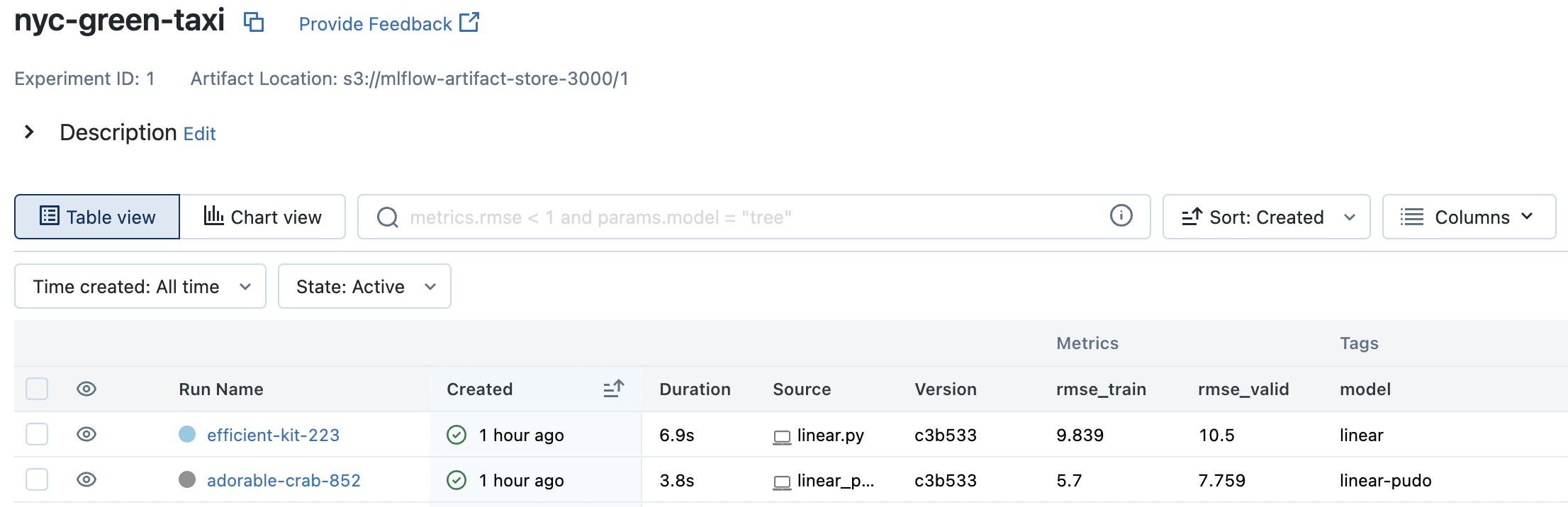
Fig. 69 Our two runs in the MLflow UI. Clicking on rmse_valid column sorts the runs based on validation RMSE.#
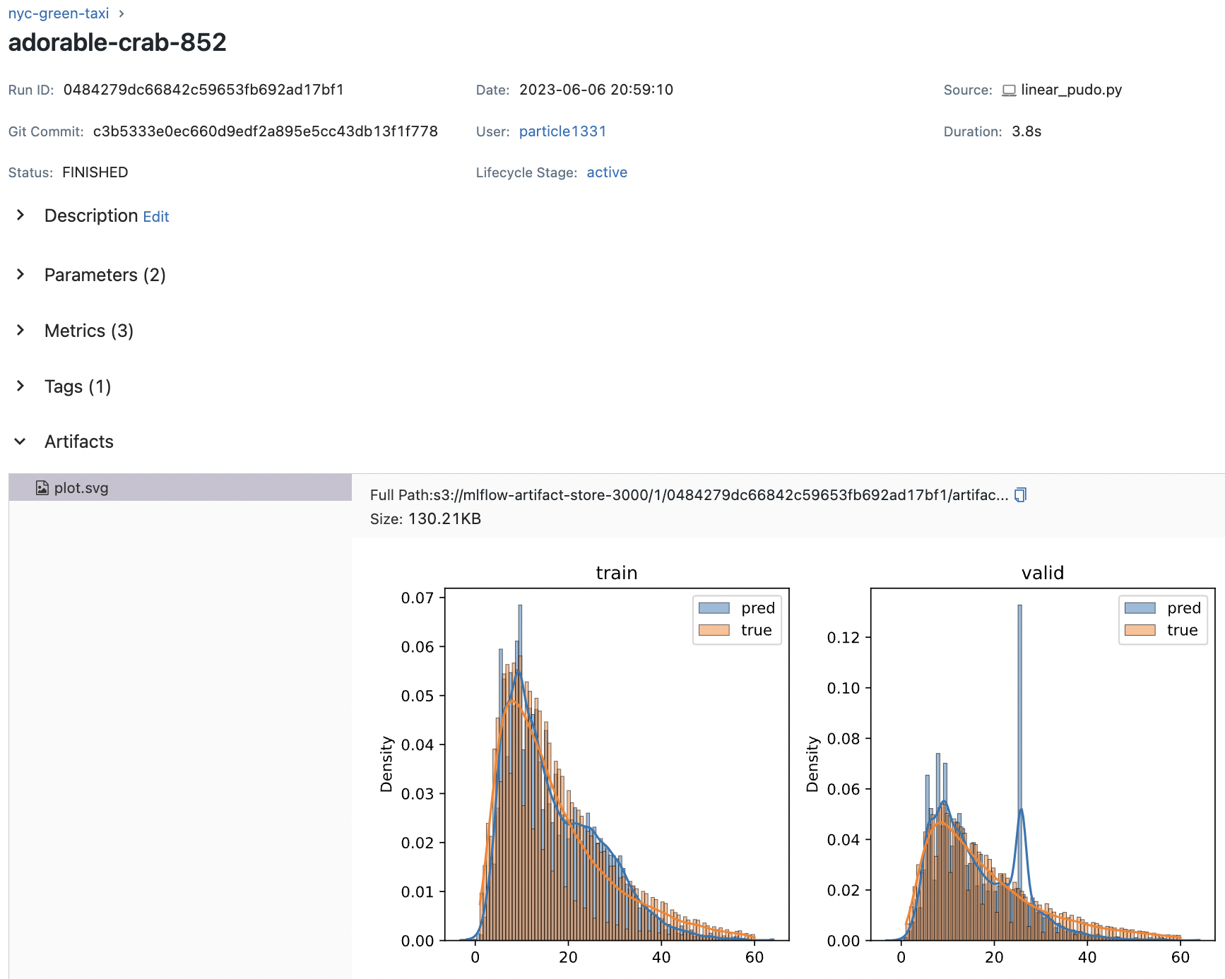
Fig. 70 Details of one run. Default parameters are logged.#
Autologging#
In this section, we show how to iterate over different models. This really just involves wrapping the run function in a loop. We also enable autologging for scikit-learn models. Automatic logging allows you to log metrics, parameters, and models without the need for explicit log statements.
# experiment/sklearn_trees.py
!pygmentize -g ~/opt/miniconda3/envs/mlops/lib/python3.9/site-packages/ride_duration/experiment/sklearn_trees.py
import os

import mlflow
from sklearn.ensemble import (
    ExtraTreesRegressor,
    RandomForestRegressor,
    GradientBoostingRegressor,
)

from ride_duration.processing import preprocess
from ride_duration.experiment.utils import (
    data_dict,
    feature_pipeline,
    setup_experiment,
    mlflow_default_logging,
)

setup_experiment()
mlflow.sklearn.autolog()  # (!)
data = data_dict(debug=int(os.environ["DEBUG"]))


def run(model_class):
    with mlflow.start_run():
        # Preprocessing
        train = data["train_data"]
        valid = data["valid_data"]
        X_train, y_train = preprocess(train, target=True, filter_target=True)
        X_valid, y_valid = preprocess(valid, target=True, filter_target=True)

        # Fit feature pipe
        feature_pipe = feature_pipeline()
        X_train = feature_pipe.fit_transform(X_train)
        X_valid = feature_pipe.transform(X_valid)

        # Fit model
        model = model_class()
        model.fit(X_train, y_train)

        # MLflow logging (default + feature pipe)
        MODEL_TAG = model_class.__name__
        args = [model, MODEL_TAG, data, X_train, y_train, X_valid, y_valid]
        mlflow_default_logging(*args)
        mlflow.sklearn.log_model(feature_pipe, "feature_pipe")


if __name__ == "__main__":
    for model_class in [
        ExtraTreesRegressor,
        GradientBoostingRegressor,
        RandomForestRegressor,
    ]:
        run(model_class)
RandomForestRegressor has the best validation score:
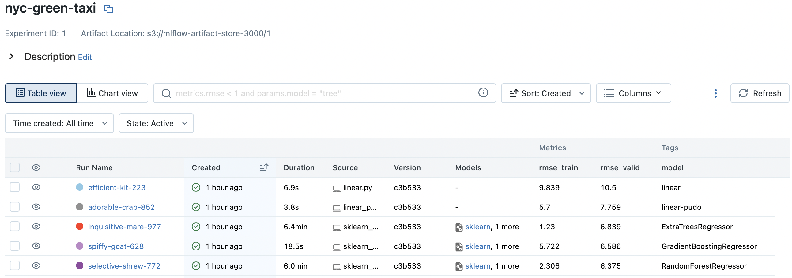
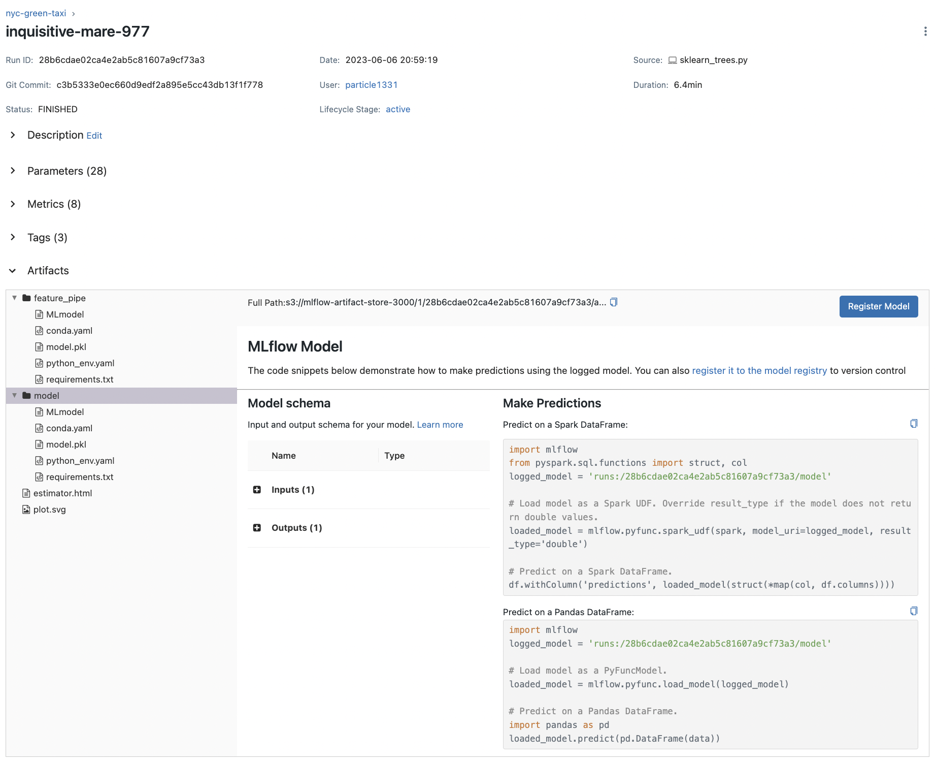
Notice an increase in parameter count which were automatically logged. Autologging also creates the MLmodel which we look at shortly (also notice Models column). It also creates config files such as conda.yaml which describe the environment used to run the scripts. This indicates the expected input and output for the model and allows easy loading as indicated:
HPO with XGBoost#
In this section, we perform hyperparameter optimization (HPO) on XGBoost using Optuna. The parameters are sampled sequentially using the TPE algorithm over the search space defined in the params dictionary. This algorithm tends to be more cost-effective than grid and random search as shown in Appendix: TPE below. Each run corresponds to a choice of hyperparameters which corresponds to a trial in the Optuna framework.
# experiment/xgboost_optuna.py
!pygmentize -g ~/opt/miniconda3/envs/mlops/lib/python3.9/site-packages/ride_duration/experiment/xgboost_optuna.py
import os

import mlflow
import optuna
from xgboost import XGBRegressor

from ride_duration.processing import preprocess
from ride_duration.experiment.utils import (
    data_dict,
    add_pudo_column,
    feature_pipeline,
    feature_selector,
    setup_experiment,
    mlflow_default_logging,
)

setup_experiment()
mlflow.xgboost.autolog()
data = data_dict(debug=int(os.environ["DEBUG"]))


def run(params: dict, pudo: int):
    with mlflow.start_run():
        # Preprocessing
        train = data["train_data"]
        valid = data["valid_data"]
        X_train, y_train = preprocess(train, target=True, filter_target=True)
        X_valid, y_valid = preprocess(valid, target=True, filter_target=True)

        # Fit feature pipe
        transforms = [add_pudo_column, feature_selector] if pudo else []
        feature_pipe = feature_pipeline(transforms)
        X_train = feature_pipe.fit_transform(X_train)
        X_valid = feature_pipe.transform(X_valid)

        # Fit model
        model = XGBRegressor(early_stopping_rounds=50, **params)
        model.fit(
            X_train,
            y_train,
            eval_set=[(X_valid, y_valid)],
        )

        # Default mlflow logs
        MODEL_TAG = "xgboost"
        args = [model, MODEL_TAG, data, X_train, y_train, X_valid, y_valid]
        logs = mlflow_default_logging(*args)

        # Logging feature pipe, use pudo
        mlflow.log_param("pudo", pudo)
        mlflow.sklearn.log_model(feature_pipe, "feature_pipe")

    return logs["rmse_valid"]


def objective(trial):
    params = {
        "max_depth": trial.suggest_int("max_depth", 4, 100),
        "n_estimators": trial.suggest_int("n_estimators", 1, 10, step=1) * 100,
        "learning_rate": trial.suggest_float("learning_rate", 1e-3, 1, log=True),
        "min_child_weight": trial.suggest_float("min_child_weight", 0.1, 300, log=True),
        "objective": "reg:squarederror",
        "seed": 42,
    }

    return run(params, pudo=trial.suggest_categorical("pudo", [0, 1]))


if __name__ == "__main__":
    import sys

    study = optuna.create_study(direction="minimize")
    study.optimize(objective, n_trials=int(sys.argv[1]))
Note that we use a flag pudo on whether to use the interaction feature between endpoint location IDs instead of each location considered separately. This is part of trial parameters so that more runs will be allocated to the setting works better with other parameters. XGBoost runs can be filtered out using tags.model = 'xgboost':
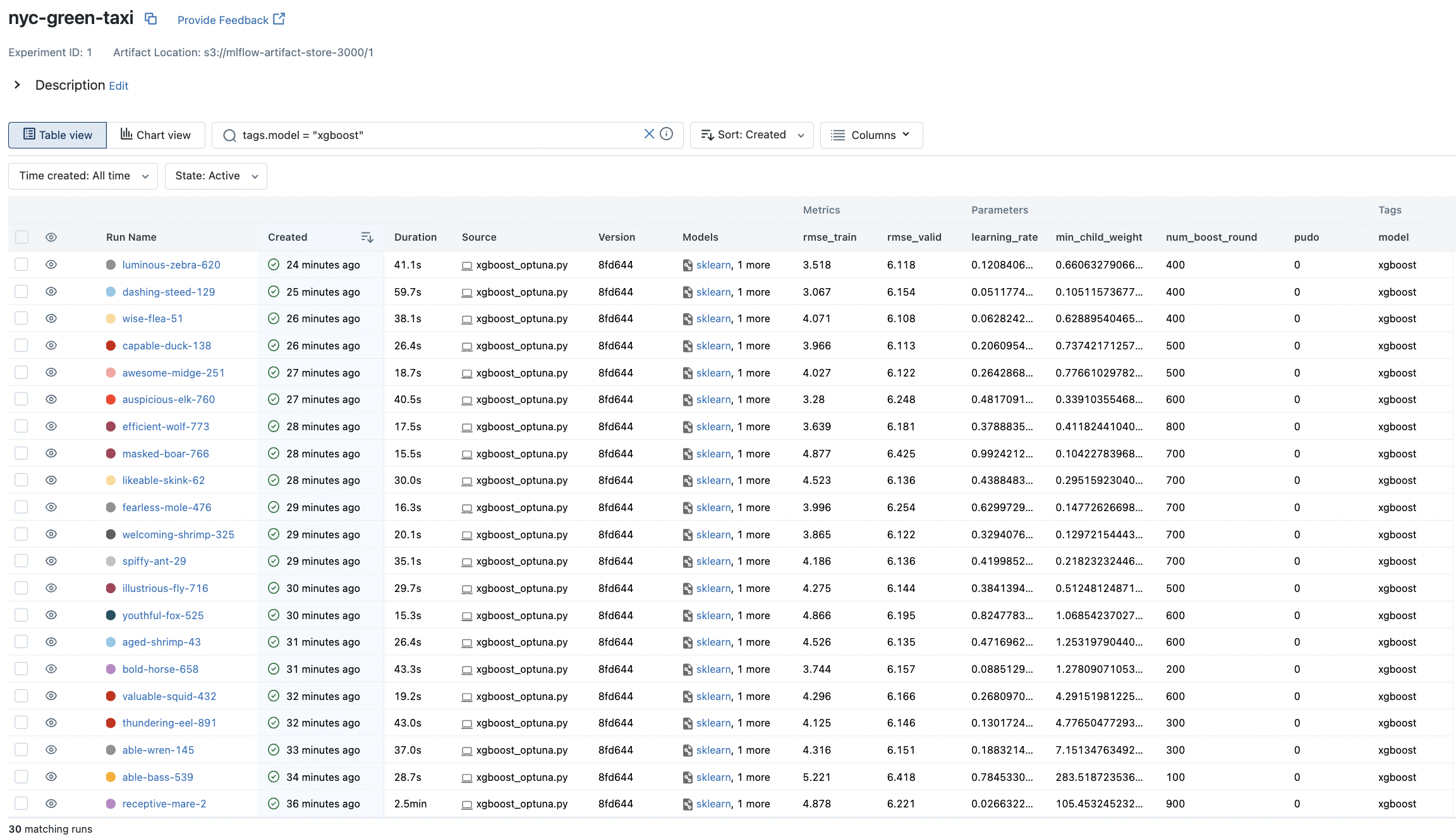
Fig. 71 Runs on the XGBoost model with autologging.#
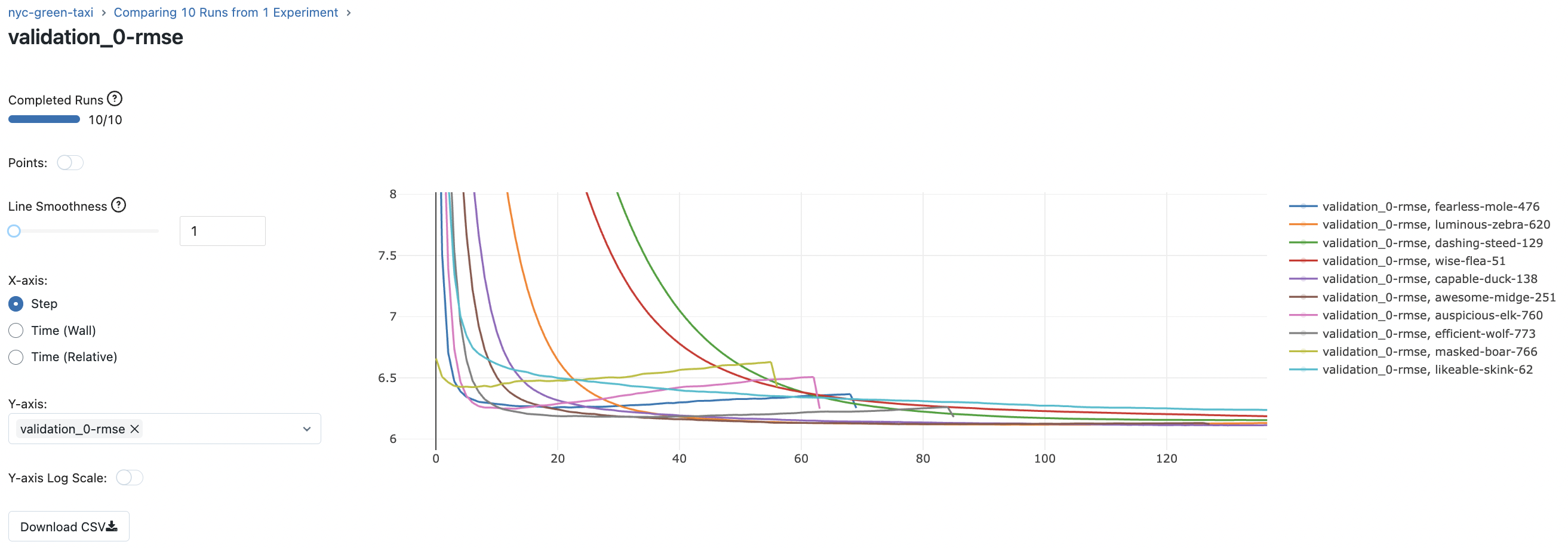
Fig. 72 Comparing validation RMSE curves for 10 runs of the XGBoost model.#
Below we look at visualizations of hyperparameter interaction:
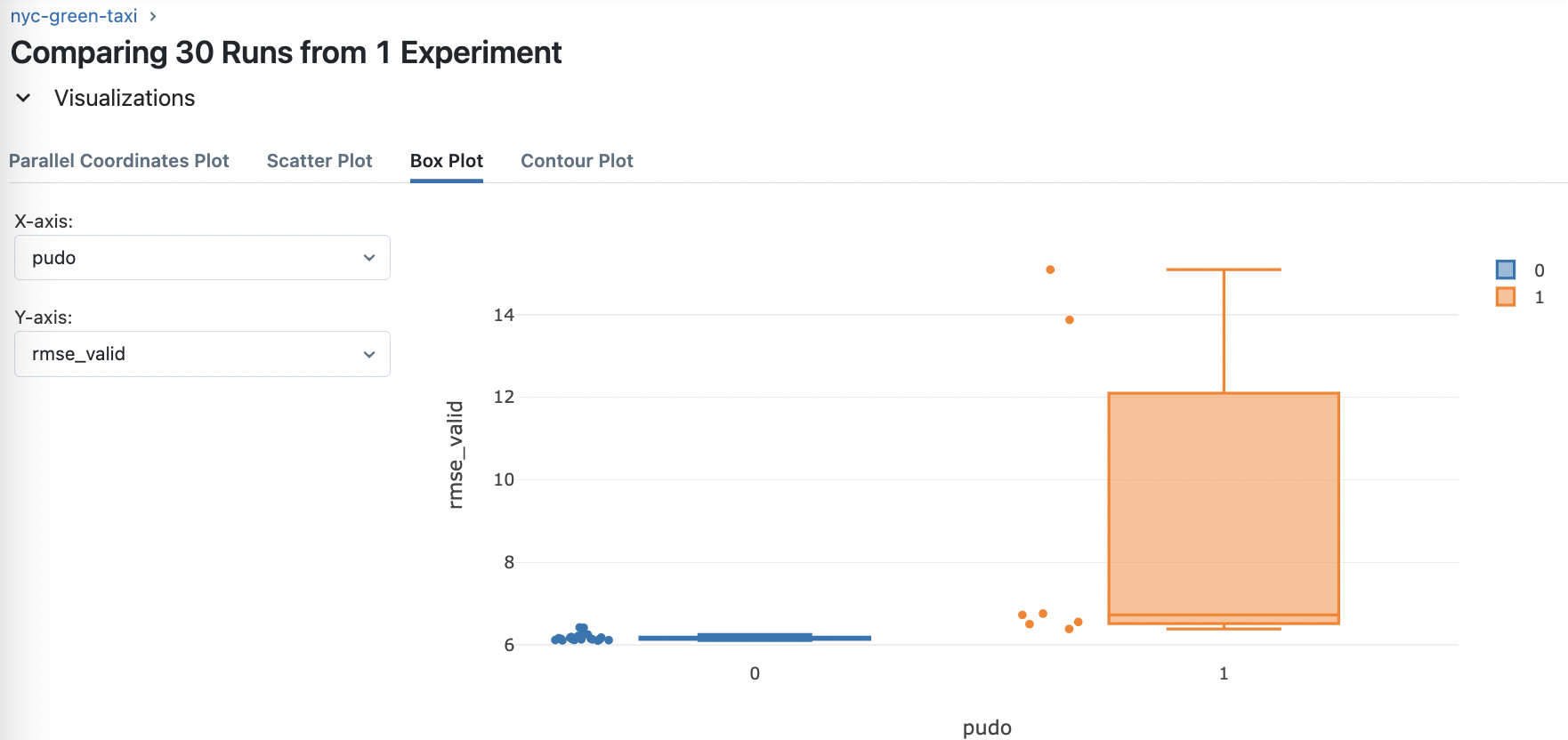
Fig. 73 Analyzing the effect of the feature engineering step of using the PU_DO column only on model performance instead of PULocationID and DOLocationID separately. Seems like not using it is better. This is a tree-based model after all.#
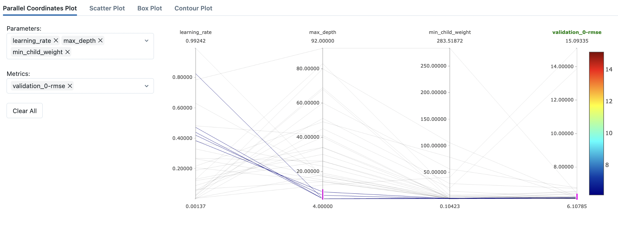
Fig. 74 Filtering out high-performing settings in the parallel coordinates plot.#
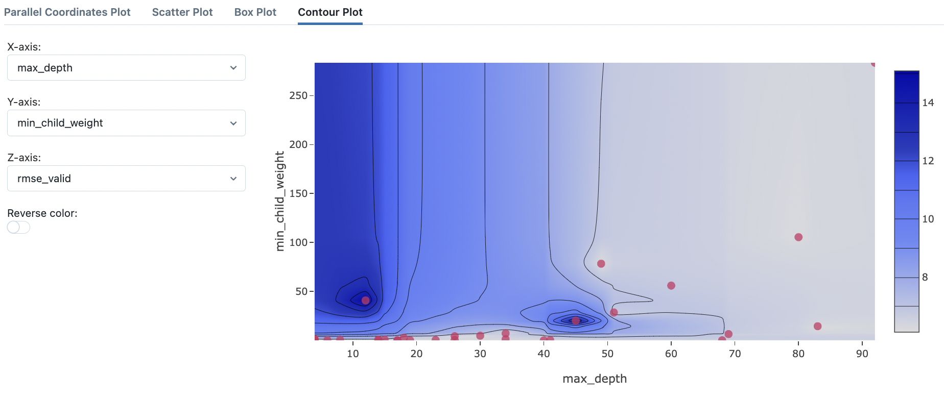
Fig. 75 Contour plot to visualize interaction of max_depth and min_child_weight.#
Model management#
Recall autologging generates an MLmodel file as well as files for approximating the environment used to generate the models. The unique run_id that corresponds to a directory in the artifacts store is assigned to each run allows for easily loading these models in remote environments. Note that even code for training these models can optionally be added as artifacts. See docs.
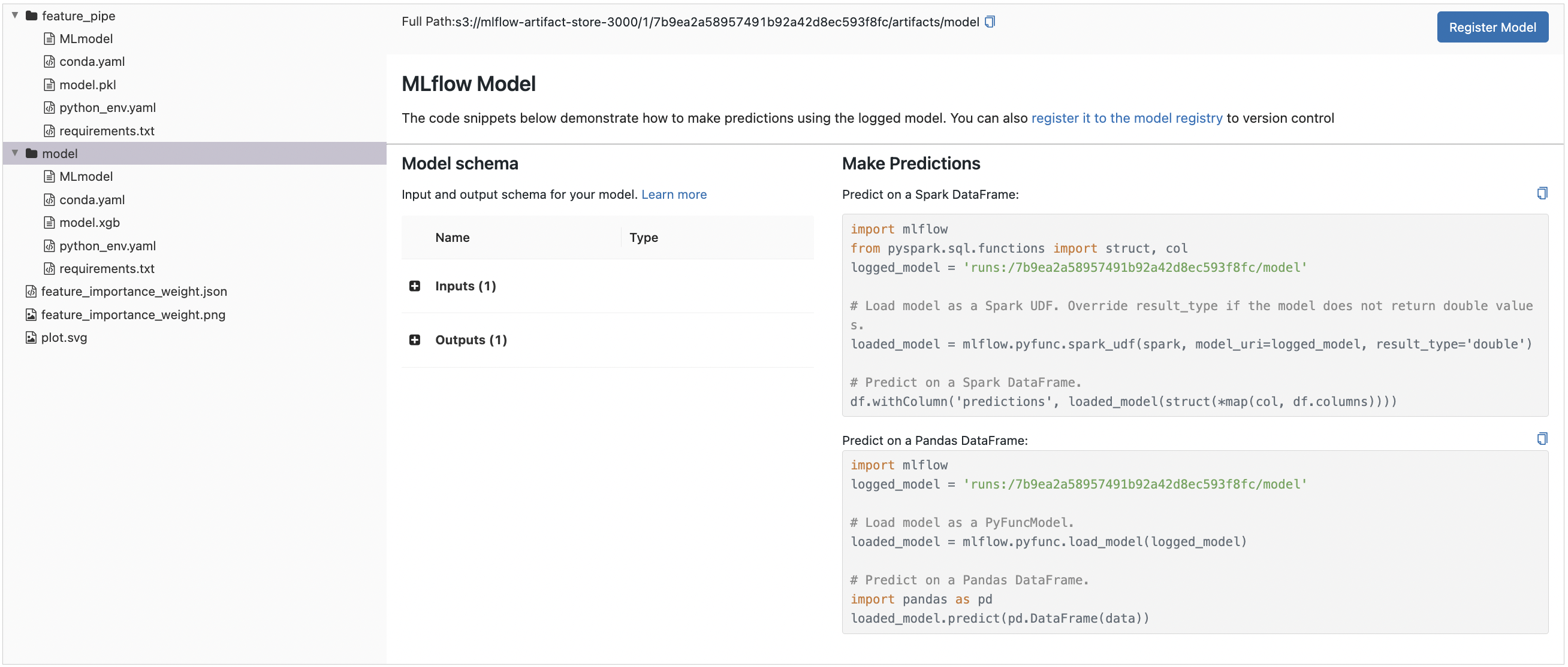
Fig. 76 MLflow model information for the XGBoost model. Note the scikit-learn based feature pipeline also has its own section. Moreover, observe that MLflow provides a uniform API for loading these models using the mlflow.pyfunc.load_model function.#
Remote model loading#
Note that a path to the model is provided above. Loading the model from S3:
import mlflow

MODEL_URI = "s3://mlflow-artifact-store-3000/1/7b9ea2a58957491b92a42d8ec593f8fc/artifacts/model"
mlflow.pyfunc.load_model(MODEL_URI)
2023/06/08 05:34:11 WARNING mlflow.pyfunc: Detected one or more mismatches between the model's dependencies and the current Python environment:
 - mlflow (current: 2.3.2, required: mlflow==2.3)
 - psutil (current: uninstalled, required: psutil==5.9.5)
To fix the mismatches, call `mlflow.pyfunc.get_model_dependencies(model_uri)` to fetch the model's environment and install dependencies using the resulting environment file.
mlflow.pyfunc.loaded_model:
  artifact_path: model
  flavor: mlflow.xgboost
  run_id: 7b9ea2a58957491b92a42d8ec593f8fc
Folder structure in S3 is as shown in the figure:
!aws s3 ls s3://mlflow-artifact-store-3000/1/7b9ea2a58957491b92a42d8ec593f8fc/artifacts/ --recursive --human-readable
2023-06-06 22:09:23    6.8 KiB 1/7b9ea2a58957491b92a42d8ec593f8fc/artifacts/feature_importance_weight.json
2023-06-06 22:09:17  320.0 KiB 1/7b9ea2a58957491b92a42d8ec593f8fc/artifacts/feature_importance_weight.png
2023-06-06 22:09:41  312 Bytes 1/7b9ea2a58957491b92a42d8ec593f8fc/artifacts/feature_pipe/MLmodel
2023-06-06 22:09:42  362 Bytes 1/7b9ea2a58957491b92a42d8ec593f8fc/artifacts/feature_pipe/conda.yaml
2023-06-06 22:09:42   14.1 KiB 1/7b9ea2a58957491b92a42d8ec593f8fc/artifacts/feature_pipe/model.pkl
2023-06-06 22:09:40  122 Bytes 1/7b9ea2a58957491b92a42d8ec593f8fc/artifacts/feature_pipe/python_env.yaml
2023-06-06 22:09:40  217 Bytes 1/7b9ea2a58957491b92a42d8ec593f8fc/artifacts/feature_pipe/requirements.txt
2023-06-06 22:09:26  676 Bytes 1/7b9ea2a58957491b92a42d8ec593f8fc/artifacts/model/MLmodel
2023-06-06 22:09:35  252 Bytes 1/7b9ea2a58957491b92a42d8ec593f8fc/artifacts/model/conda.yaml
2023-06-06 22:09:27    9.2 MiB 1/7b9ea2a58957491b92a42d8ec593f8fc/artifacts/model/model.xgb
2023-06-06 22:09:25  122 Bytes 1/7b9ea2a58957491b92a42d8ec593f8fc/artifacts/model/python_env.yaml
2023-06-06 22:09:26  127 Bytes 1/7b9ea2a58957491b92a42d8ec593f8fc/artifacts/model/requirements.txt
2023-06-06 22:09:37  128.9 KiB 1/7b9ea2a58957491b92a42d8ec593f8fc/artifacts/plot.svg
The feature pipeline can therefore be loaded similarly:
ARTIFACTS_STORE  = "s3://mlflow-artifact-store-3000"
EXPERIMENT_ID    = "1"
RUN_ID           = "7b9ea2a58957491b92a42d8ec593f8fc"
ARTIFACTS_PATH   = f"{ARTIFACTS_STORE}/{EXPERIMENT_ID}/{RUN_ID}/artifacts"
MODEL_URI        = f"{ARTIFACTS_PATH}/model"
FEATURE_PIPE_URI = f"{ARTIFACTS_PATH}/feature_pipe"

# Loading models from S3
model = mlflow.pyfunc.load_model(MODEL_URI)
feature_pipe = mlflow.sklearn.load_model(FEATURE_PIPE_URI)
2023/06/08 05:34:33 WARNING mlflow.pyfunc: Detected one or more mismatches between the model's dependencies and the current Python environment:
 - mlflow (current: 2.3.2, required: mlflow==2.3)
 - psutil (current: uninstalled, required: psutil==5.9.5)
To fix the mismatches, call `mlflow.pyfunc.get_model_dependencies(model_uri)` to fetch the model's environment and install dependencies using the resulting environment file.
The models can then be used to make inference:
import pandas as pd
from sklearn.metrics import mean_squared_error
from ride_duration.processing import preprocess

# Load data from some data source
data = pd.read_parquet("data/green_tripdata_2021-02.parquet")

# Inference on validation data
X, y = preprocess(data, target=True, filter_target=True)
X = feature_pipe.transform(X)
y_pred = model.predict(X)
print(mean_squared_error(y, y_pred) ** 0.5) # Expected: ~6.108
6.107853695857164
Remark. The same code can be used to make inference using any other model trained in the nyc-green-taxi experiment (i.e. pyfunc models with a .predict() method). Note that feature engineering steps are baked into the feature_pipe model so that this script is fairly general.
Model registry#
Consider the scenario where a member of our team chooses a new model for production. As deployment engineers, we naturally have the following questions in mind: What has changed in this new model? Is there any preprocessing needed? What are the dependencies? Without experiment tracking, this requires a lot of back and fort communication. If there is an incident and we had to rollback the model version, we have to manually trace what changed in this new version. Moreover, it might not be possible to get back the previous model as information of how it was trained has been lost.
Our tracking database and standard model files, solves most of these issues. Having a model registry takes care of the last details of model release and staging. If we want to rollback models, we only have to look at the archived models, or earlier versions, which also have their own model lineage. It is also natural to update models trained on the same task since models typically degrades with time or improve with new techniques so that registering a model with multiple versions that correspond to runs make sense.

Fig. 77 Registering models into stages allows identification for QA and downstream tasks.#
Suppose we need fast models. We can take the Pareto front of predict time and validation RMSE. Also taking the nearest model on the right which has better RMSE but is about 10x slower. We imagine this to be an update to the first model.
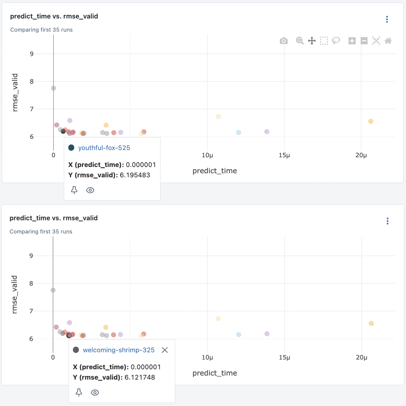
Fig. 78 Two models at the Pareto front of valid RMSE and predict time.#
Registering this model can be done by simply clicking the “Register Model” button in the UI. We choose the name NYCGreenTaxiRideDuration and we stage the first model in production. The latter model is set to staging. The model registry can be viewed in the Models tab of the UI.
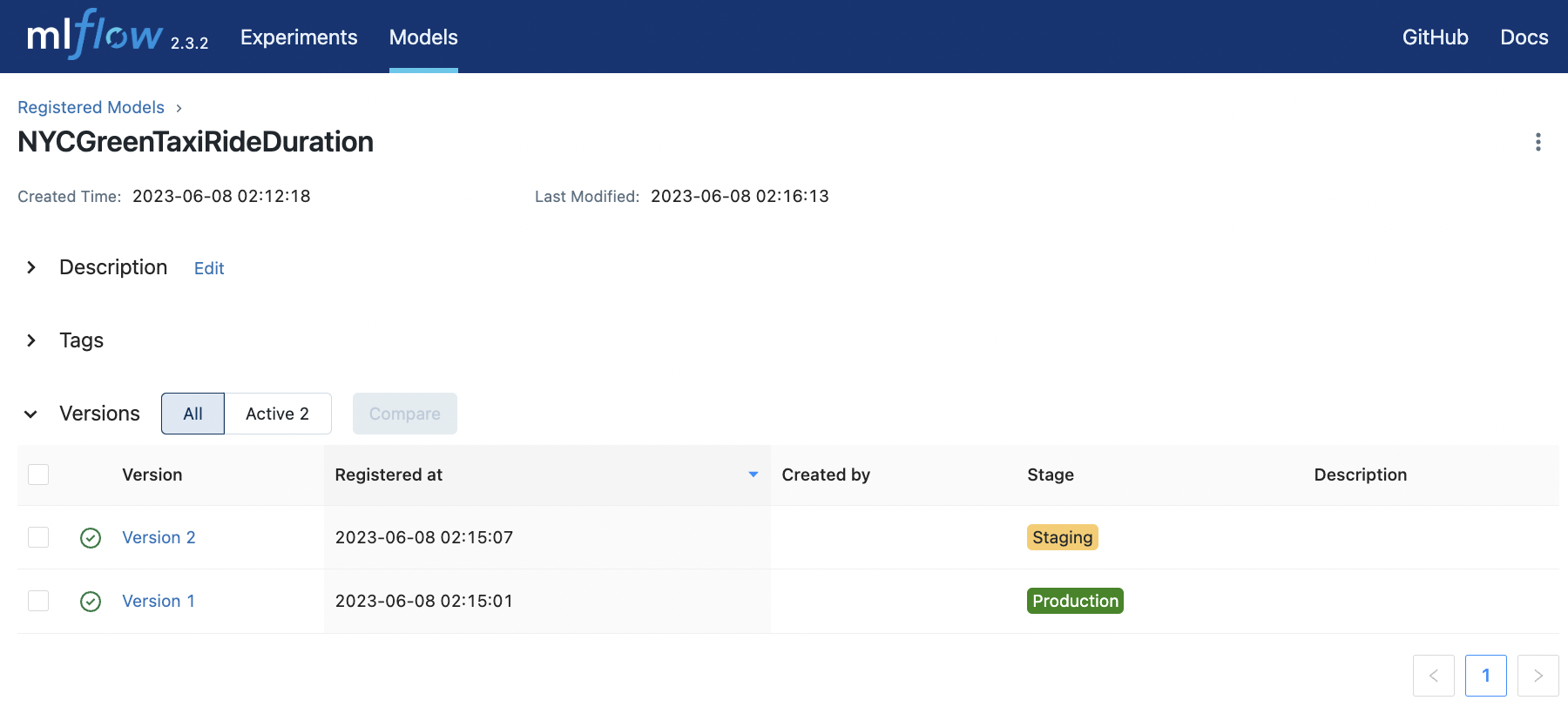
Fig. 79 Registering a model and staging a new version of the model trained on the same task.#
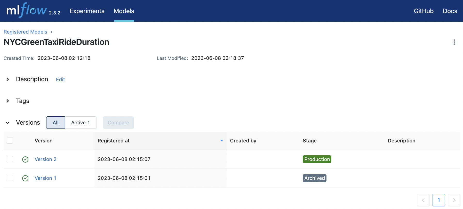
Fig. 80 Transitioning the staged model to production and the current prod model to archived.#
Remark. Note that experiment runs does not always need to involve model training. It can consist of evaluation (e.g. for large pretrained models) on a variety of tasks or datasets. So model versions here can consist of different versions of a pretrained model or different sizes of an LLM.
API Workflows#
In this section, we look at how to programatically interact with the MLflow server through its client. The idea is that everything that we can do in the UI by clicking buttons, we should be able to do here in code. And the fields that are available using the UI correspond to function arguments of the corresponding API endpoint or client method.
Experiment tracking#
The MlflowClient connects to the experiment tracking server. This provides a CRUD interface for managing experiments and runs. For example, we can list all experiments:
from mlflow.tracking import MlflowClient

TRACKING_URI = "http://127.0.0.1:5001"
client = MlflowClient(tracking_uri=TRACKING_URI)

def print_experiment(experiment):
    print(f"(Experiment)")
    print(f"    experiment_id={experiment.experiment_id}")
    print(f"    name='{experiment.name}'")
    print(f"    artifact_location='{experiment.artifact_location}'")
    print()


for experiment in client.search_experiments():
    print_experiment(experiment)
(Experiment)
    experiment_id=1
    name='nyc-green-taxi'
    artifact_location='s3://mlflow-artifact-store-3000/1'

(Experiment)
    experiment_id=0
    name='Default'
    artifact_location='s3://mlflow-artifact-store-3000/0'
Remark. Here we have the SQLite file mlflow.db on disk. In practice, you may have a remote tracking database (see Appendix). But the overall idea is the same — only the URI changes.
In the previous section, we selected two best performing runs using the UI. This can be done with the client using the search_runs method. Note that MLflow stores even deleted experiments. So we specify ViewType to ACTIVE_ONLY in the search results.
from mlflow.entities import ViewType

runs = client.search_runs(
    experiment_ids=1,
    filter_string='metrics.predict_time < 3e-6 and metrics.predict_time < 6.20',
    run_view_type=ViewType.ACTIVE_ONLY,
    max_results=15,
    order_by=["metrics.rmse_valid ASC", "metrics.predict_time ASC"]
)

for run in runs:
    name = run.info.run_name
    format_name = name + " " * (16 - len(name)) if len(name) <= 16 else name[:13] + "..."
    print(f"{format_name}  {run.info.run_id}  rmse_valid: {run.data.metrics['rmse_valid']:.3f}  predict_time: {run.data.metrics['predict_time']:.4e}")
capable-duck-138  ab1627e83ba54533a6cef8808fffa833  rmse_valid: 6.113  predict_time: 1.9263e-06
welcoming-shr...  3b22785082064008970cca22d9437fc9  rmse_valid: 6.122  predict_time: 1.0417e-06
awesome-midge...  0dd2282af2ee4285883496f85de5391d  rmse_valid: 6.122  predict_time: 1.1373e-06
aged-shrimp-43    011a2ceeffd8456b9efe40c607fb316b  rmse_valid: 6.135  predict_time: 2.0041e-06
likeable-skin...  6b6d237b07124a18a5209a58644aa212  rmse_valid: 6.136  predict_time: 1.7963e-06
spiffy-ant-29     b94a01e596f04b18bef92ba57311558e  rmse_valid: 6.136  predict_time: 1.9076e-06
illustrious-f...  b4a2096903bc45349c8a7d157e3824d7  rmse_valid: 6.144  predict_time: 1.2170e-06
valuable-squi...  33e47ef0f9b44e92ab650aaf3e941e55  rmse_valid: 6.166  predict_time: 1.2816e-06
efficient-wol...  0235a03362a2467b8713b4598487182d  rmse_valid: 6.181  predict_time: 9.8972e-07
youthful-fox-525  a80338fa398e466ca80190b02c4a4923  rmse_valid: 6.195  predict_time: 6.3362e-07
auspicious-el...  c18f4798677241158c795d863e10b408  rmse_valid: 6.248  predict_time: 7.6249e-07
fearless-mole...  2e765f99f8274f6680e696235e80615f  rmse_valid: 6.254  predict_time: 4.5257e-07
masked-boar-766   0cf15c3481c44da4a15495a49848dad5  rmse_valid: 6.425  predict_time: 2.0791e-07
spiffy-goat-628   990a81c769944bfab8f7608b520ba24d  rmse_valid: 6.586  predict_time: 1.0645e-06
adorable-crab...  0484279dc66842c59653fb692ad17bf1  rmse_valid: 7.759  predict_time: 3.3842e-09
Remark. This may give us better results than visual inspection when choosing models.
Model registry#
Creating a new model version. Note that if the name does not exist, it registers a new model with the source run as initial version.
import mlflow

# First run in our above query
RUN_ID = runs[0].info.run_id
MODEL_URI = f"s3://mlflow-artifact-store-3000/1/{RUN_ID}/artifacts/model"

client.create_model_version(
    name="NYCGreenTaxiRideDuration",
    run_id=RUN_ID,
    source=MODEL_URI
);
2023/06/08 05:35:28 INFO mlflow.tracking._model_registry.client: Waiting up to 300 seconds for model version to finish creation. Model name: NYCGreenTaxiRideDuration, version 3
This version can be transitioned to staging as follows:
import datetime
def transition_stage(client, model_name, version, stage, archive_existing=False):
"""Transition model version to given stage. Log update in description."""
client.transition_model_version_stage(
name=model_name,
version=version,
stage=stage,
archive_existing_versions=archive_existing
)
t = datetime.datetime.now()
s = t.isoformat(timespec="seconds")
description = client.get_model_version(model_name, version).description or ""
client.update_model_version(
name=model_name,
version=version,
description=(
f"[{s}] Model version transitioned to {stage}.\n"
f"{description}"
)
)
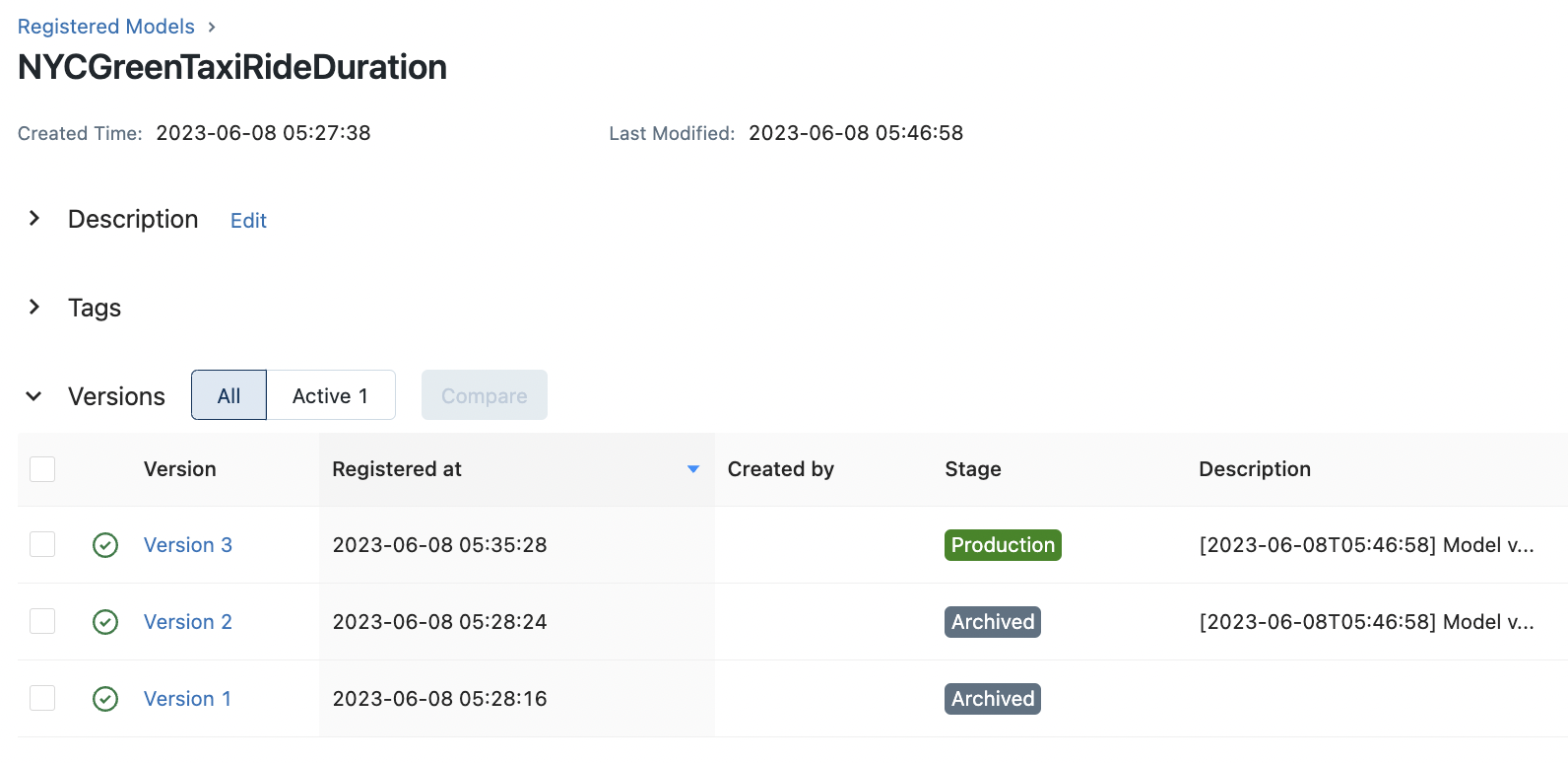
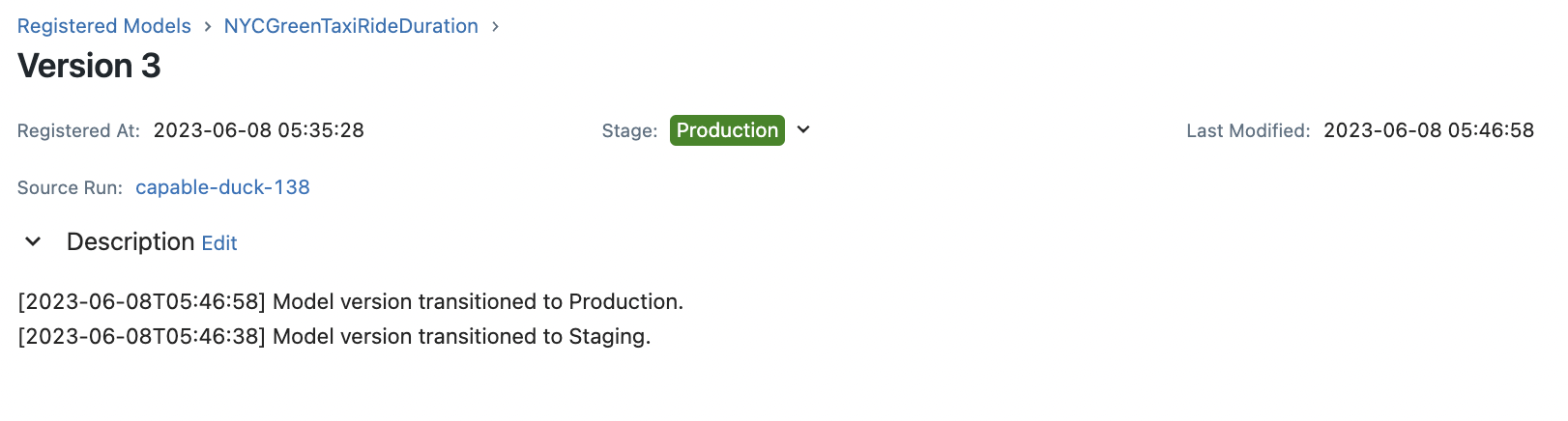
transition_stage(client, "NYCGreenTaxiRideDuration", 3, "Staging")
The following lists the latest versions for each stage:
latest_versions = client.get_latest_versions(name="NYCGreenTaxiRideDuration")
for version in latest_versions:
    print(f"Version: {version.version}   Run ID: {version.run_id}   Stage: {version.current_stage}" )
Version: 1   Run ID: a80338fa398e466ca80190b02c4a4923   Stage: Archived
Version: 2   Run ID: 3b22785082064008970cca22d9437fc9   Stage: Production
Version: 3   Run ID: ab1627e83ba54533a6cef8808fffa833   Stage: Staging
The same transition function can be used to promote v4 to production and archive v3 which is currently in production. Note that we can automatically archive v2 using archive_existing=True. But we use the transition function so that the transition is logged in the description.
transition_stage(client, "NYCGreenTaxiRideDuration", 3, "Production")
transition_stage(client, "NYCGreenTaxiRideDuration", 2, "Archived")
Inference with staged models#
Here we load the latest production model from S3:
MODEL_NAME = "NYCGreenTaxiRideDuration"
STAGE      = "Production"

RUN_ID = client.get_latest_versions(name=MODEL_NAME, stages=[STAGE])[0].run_id

ARTIFACTS_PATH   = f"{ARTIFACTS_STORE}/{EXPERIMENT_ID}/{RUN_ID}/artifacts"
MODEL_URI        = f"{ARTIFACTS_PATH}/model"
FEATURE_PIPE_URI = f"{ARTIFACTS_PATH}/feature_pipe"


# Loading models from S3
model = mlflow.pyfunc.load_model(MODEL_URI)
feature_pipe = mlflow.sklearn.load_model(FEATURE_PIPE_URI)

# Load data from some data source
data = pd.read_parquet("data/green_tripdata_2021-02.parquet")

# Inference on validation data
X, y = preprocess(data, target=True, filter_target=True)
X = feature_pipe.transform(X)
y_pred = model.predict(X)
print(mean_squared_error(y, y_pred) ** 0.5)
2023/06/08 05:52:25 WARNING mlflow.pyfunc: Detected one or more mismatches between the model's dependencies and the current Python environment:
 - mlflow (current: 2.3.2, required: mlflow==2.3)
 - psutil (current: uninstalled, required: psutil==5.9.5)
To fix the mismatches, call `mlflow.pyfunc.get_model_dependencies(model_uri)` to fetch the model's environment and install dependencies using the resulting environment file.
6.112723434664211
Expected:
client.get_run(RUN_ID).data.metrics["rmse_valid"]
6.112723434664211
Remark. MLflow seems to like working with latest versions in the registry by default. This makes sense. But a workaround to getting all models at a given stage is the following (sorted by latest at index 0).
from datetime import datetime

STAGE = "Archived"
runs = client.search_model_versions(f"name='{MODEL_NAME}'")

print(f"({MODEL_NAME})")
print(f"Stage: {STAGE}")
for run in runs:
    if run.current_stage == STAGE:
        last_updated = run.last_updated_timestamp / 1000    # ms
        print("\n  Version:", run.version)
        print("  Run ID:", run.run_id)
        print("  Status:", run.status)
        print("  Last Modified:", datetime.fromtimestamp(last_updated).strftime('%Y-%m-%d %H:%M:%S'))
(NYCGreenTaxiRideDuration)
Stage: Archived

  Version: 2
  Run ID: 3b22785082064008970cca22d9437fc9
  Status: READY
  Last Modified: 2023-06-08 05:46:58

  Version: 1
  Run ID: a80338fa398e466ca80190b02c4a4923
  Status: READY
  Last Modified: 2023-06-08 05:33:36
Appendix: TPE algorithm#
Samplers which determine the sequence of trials are specified when creating a Optuna study:
study = create_study(
    direction="maximize",
    sampler=optuna.samplers.TPESampler()
)
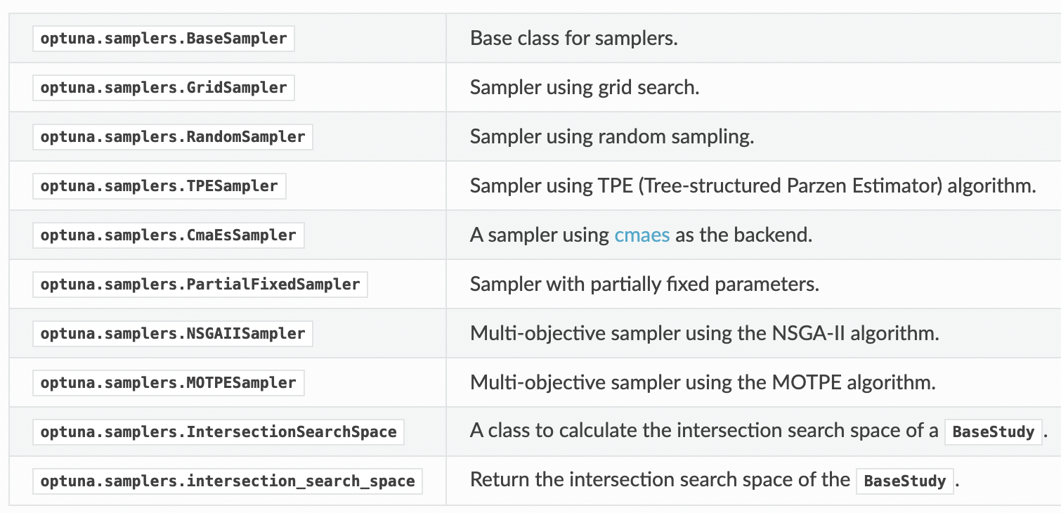
Fig. 81 List of all sampling algorithms as of version 2.10.0.#
Optuna uses Tree-Structured Parzen Estimater (TPE) [BBBK11] as the default sampler. This algorithm estimates the probability density of each parameter independently:
On each trial, for each parameter, TPE fits one Gaussian Mixture Model (GMM)
l(x)to the set of parameter values associated with the best objective values, and another GMMg(x)to the remaining parameter values. It chooses the parameter valuexthat maximizes the ratiol(x)/g(x). — (optuna.samplers.TPESampler)
In general, we expect TPE to be more efficient than random search. To demonstrate TPE, we minimize the following objective function:
Show code cell content
import numpy as np
import matplotlib.pyplot as plt
from matplotlib import cm

%matplotlib inline
import matplotlib_inline
matplotlib_inline.backend_inline.set_matplotlib_formats('svg')


def plot_contour(f, title, ax, x_range, y_range, cmap=cm.cividis):
    """Generate 2d contour plot of function f with two parameters."""

    # Plot surface on xy plane; choose 3d or 2d plot
    x = np.linspace(x_range[0], x_range[1], 100)
    y = np.linspace(y_range[0], y_range[1], 100)
    X, Y = np.meshgrid(x, y)
    Z = f(X, Y)

    # Plot
    ax.contourf(X, Y, Z, cmap=cmap)
    ax.set_xlim(x_range)
    ax.set_ylim(y_range)
    ax.set_title(title)
    ax.set_xlabel(r"$w_1$")
    ax.set_ylabel(r"$w_2$")
    return ax


def plot_surface(f, title, ax, x_range, y_range, cmap=cm.viridis):
    """Generate 3d surface plot {(x, y, f(x, y)) | x ∈ x_range, y ∈ y_range}."""

    # Plot surface on xy plane; choose 3d or 2d plot
    x = np.linspace(x_range[0], x_range[1], 100)
    y = np.linspace(y_range[0], y_range[1], 100)
    X, Y = np.meshgrid(x, y)
    Z = f(X, Y)

    # Plot
    ax.plot_surface(X, Y, Z, cmap=cmap, linewidth=1, color="#000", antialiased=False)
    ax.set_zlabel("loss", rotation=90)

    # Formatting plot
    plt.xlim(x_range)
    plt.ylim(y_range)
    plt.title(title)
    ax.set_xlabel(r"$x$")
    ax.set_ylabel(r"$y$")
    plt.tight_layout()

    return ax


def plot_results(study, ax, p1, p2, f, x_range, y_range, figsize=(8, 5)):
    """Scatter plot optimization steps with contour in background."""

    plot_contour(f, "objective", ax=ax, x_range=x_range, y_range=y_range)
    study.trials_dataframe().plot(
        kind='scatter',
        ax=ax,
        figsize=figsize,
        color='C3', edgecolor='black',
        x='params_'+p1, y='params_'+p2,
        xlabel=p1, ylabel=p2
    )
    plt.axis("equal")
def f(x, y):
    """Flat surface with three holes."""
    r = 4.0
    center = [(0, 0), (3, 3), (6, -3)]
    factor = [-5.0, -4.5, -4.8]
    for j, c in enumerate(center):
        r += factor[j] * np.exp(-(x - c[0])**2 - (y - c[1])**2)
    return r


fig = plt.figure(figsize=(5, 5))
ax = fig.add_subplot(projection='3d')
plot_surface(f, title="Objective", x_range=(-4, 10), y_range=(-6, 6), ax=ax);

Note that from the color of the surface that we get better minimas for decreasing \(\mathsf x.\)
import optuna

def objective(trial):
    x = trial.suggest_float('x', -4, 10)
    y = trial.suggest_float('y', -6,  6)
    return f(x, y)


min_f = optuna.create_study(direction="minimize")
min_f.optimize(objective, n_trials=50) # TPE default sampler
Show code cell output
/Users/particle1331/opt/miniconda3/envs/mlops/lib/python3.9/site-packages/tqdm/auto.py:21: TqdmWarning: IProgress not found. Please update jupyter and ipywidgets. See https://ipywidgets.readthedocs.io/en/stable/user_install.html
  from .autonotebook import tqdm as notebook_tqdm
[I 2023-06-08 02:39:56,199] A new study created in memory with name: no-name-3a96122b-a3f6-4fa8-9486-14c97346bddc
[I 2023-06-08 02:39:56,202] Trial 0 finished with value: 3.7573587447494186 and parameters: {'x': 5.507005301522042, 'y': -4.6558210614366695}. Best is trial 0 with value: 3.7573587447494186.
[I 2023-06-08 02:39:56,203] Trial 1 finished with value: 3.0557035559333294 and parameters: {'x': 1.1332522374715532, 'y': 0.6188670535764764}. Best is trial 1 with value: 3.0557035559333294.
[I 2023-06-08 02:39:56,204] Trial 2 finished with value: 3.9999977020278723 and parameters: {'x': -3.7751684586695724, 'y': -0.583973054775683}. Best is trial 1 with value: 3.0557035559333294.
[I 2023-06-08 02:39:56,204] Trial 3 finished with value: 3.9999974830659144 and parameters: {'x': 0.155083854817903, 'y': 5.5105773597663354}. Best is trial 1 with value: 3.0557035559333294.
[I 2023-06-08 02:39:56,205] Trial 4 finished with value: 3.999999999007288 and parameters: {'x': 9.900785441018803, 'y': -0.33859634067690436}. Best is trial 1 with value: 3.0557035559333294.
[I 2023-06-08 02:39:56,205] Trial 5 finished with value: 3.999999999998051 and parameters: {'x': 7.498749921833506, 'y': 5.86860562331367}. Best is trial 1 with value: 3.0557035559333294.
[I 2023-06-08 02:39:56,206] Trial 6 finished with value: 3.9999999999770037 and parameters: {'x': -3.705602171126929, 'y': 3.5176194025812784}. Best is trial 1 with value: 3.0557035559333294.
[I 2023-06-08 02:39:56,207] Trial 7 finished with value: 3.9996992711194355 and parameters: {'x': 2.96287708877078, 'y': -3.6736507204867404}. Best is trial 1 with value: 3.0557035559333294.
[I 2023-06-08 02:39:56,207] Trial 8 finished with value: 3.98888013968075 and parameters: {'x': 4.971397128724682, 'y': 4.4548860124042235}. Best is trial 1 with value: 3.0557035559333294.
[I 2023-06-08 02:39:56,208] Trial 9 finished with value: 3.9527734218589012 and parameters: {'x': 0.9840265675958539, 'y': 3.7019771240800434}. Best is trial 1 with value: 3.0557035559333294.
[I 2023-06-08 02:39:56,215] Trial 10 finished with value: 2.460459178155704 and parameters: {'x': -0.45633882256921243, 'y': 0.9847379923495998}. Best is trial 10 with value: 2.460459178155704.
[I 2023-06-08 02:39:56,222] Trial 11 finished with value: 3.761681754171921 and parameters: {'x': 0.05158941659008387, 'y': 1.744012324771865}. Best is trial 10 with value: 2.460459178155704.
[I 2023-06-08 02:39:56,228] Trial 12 finished with value: 3.917068608084295 and parameters: {'x': -1.6355745486634166, 'y': 1.1933463141936165}. Best is trial 10 with value: 2.460459178155704.
[I 2023-06-08 02:39:56,235] Trial 13 finished with value: 3.9994662880949434 and parameters: {'x': 2.3736861306573185, 'y': -1.875007597676755}. Best is trial 10 with value: 2.460459178155704.
[I 2023-06-08 02:39:56,241] Trial 14 finished with value: 3.9380945020847364 and parameters: {'x': -1.4885531868446968, 'y': 1.4750571578537521}. Best is trial 10 with value: 2.460459178155704.
[I 2023-06-08 02:39:56,247] Trial 15 finished with value: 3.9807605489341795 and parameters: {'x': 1.5942609068678557, 'y': -1.7374011144228312}. Best is trial 10 with value: 2.460459178155704.
[I 2023-06-08 02:39:56,254] Trial 16 finished with value: 3.995224701293237 and parameters: {'x': -1.1823805497629638, 'y': 2.357059326842403}. Best is trial 10 with value: 2.460459178155704.
[I 2023-06-08 02:39:56,261] Trial 17 finished with value: 3.9607291280178814 and parameters: {'x': 2.909265302097056, 'y': 0.8212630989407523}. Best is trial 10 with value: 2.460459178155704.
[I 2023-06-08 02:39:56,268] Trial 18 finished with value: 3.8158404791348906 and parameters: {'x': 1.2382814293962208, 'y': 2.6891531969150524}. Best is trial 10 with value: 2.460459178155704.
[I 2023-06-08 02:39:56,275] Trial 19 finished with value: 3.995038588189308 and parameters: {'x': 4.0958742273650985, 'y': 0.6316070291771115}. Best is trial 10 with value: 2.460459178155704.
[I 2023-06-08 02:39:56,283] Trial 20 finished with value: 0.11743765148144163 and parameters: {'x': -0.32300730865073213, 'y': -0.38549819249544415}. Best is trial 20 with value: 0.11743765148144163.
[I 2023-06-08 02:39:56,290] Trial 21 finished with value: -0.8496512838581487 and parameters: {'x': 0.16852102536102198, 'y': -0.046171450878570885}. Best is trial 21 with value: -0.8496512838581487.
[I 2023-06-08 02:39:56,298] Trial 22 finished with value: 2.1858965427387864 and parameters: {'x': -0.36798123152400963, 'y': -0.9372493493997028}. Best is trial 21 with value: -0.8496512838581487.
[I 2023-06-08 02:39:56,307] Trial 23 finished with value: 3.9977412902087375 and parameters: {'x': -2.282482952211657, 'y': -1.5788194965974482}. Best is trial 21 with value: -0.8496512838581487.
[I 2023-06-08 02:39:56,316] Trial 24 finished with value: 0.852095960181563 and parameters: {'x': -0.23722990543001782, 'y': -0.6375131663653602}. Best is trial 21 with value: -0.8496512838581487.
[I 2023-06-08 02:39:56,324] Trial 25 finished with value: 3.999966965095532 and parameters: {'x': -2.0598599211571518, 'y': -2.7720679757136235}. Best is trial 21 with value: -0.8496512838581487.
[I 2023-06-08 02:39:56,333] Trial 26 finished with value: 3.906280991396571 and parameters: {'x': 1.9947599575179455, 'y': 0.001341755447659465}. Best is trial 21 with value: -0.8496512838581487.
[I 2023-06-08 02:39:56,342] Trial 27 finished with value: 3.9999999999999867 and parameters: {'x': 0.4948746367736898, 'y': -5.771107052068123}. Best is trial 21 with value: -0.8496512838581487.
[I 2023-06-08 02:39:56,350] Trial 28 finished with value: 2.8793900639210093 and parameters: {'x': -0.6435702445203852, 'y': -1.0398952495053733}. Best is trial 21 with value: -0.8496512838581487.
[I 2023-06-08 02:39:56,357] Trial 29 finished with value: 3.9912988809872854 and parameters: {'x': -2.5159342864331027, 'y': 0.1543250408264475}. Best is trial 21 with value: -0.8496512838581487.
[I 2023-06-08 02:39:56,364] Trial 30 finished with value: 3.999310837229508 and parameters: {'x': 0.49965418854147803, 'y': -2.9393565074721506}. Best is trial 21 with value: -0.8496512838581487.
[I 2023-06-08 02:39:56,372] Trial 31 finished with value: 2.572433707184051 and parameters: {'x': -0.5267124129385377, 'y': -0.9879477947854147}. Best is trial 21 with value: -0.8496512838581487.
[I 2023-06-08 02:39:56,380] Trial 32 finished with value: 0.6891176201197601 and parameters: {'x': -0.6301510495356093, 'y': -0.12301558220649716}. Best is trial 21 with value: -0.8496512838581487.
[I 2023-06-08 02:39:56,388] Trial 33 finished with value: 2.292336086978142 and parameters: {'x': 1.0305217152646893, 'y': 0.11112848163080308}. Best is trial 21 with value: -0.8496512838581487.
[I 2023-06-08 02:39:56,395] Trial 34 finished with value: 2.663353039500105 and parameters: {'x': -1.1394264770120155, 'y': -0.14484821763047379}. Best is trial 21 with value: -0.8496512838581487.
[I 2023-06-08 02:39:56,402] Trial 35 finished with value: 3.9211842816849827 and parameters: {'x': 1.9372874234393356, 'y': -0.6301056444537388}. Best is trial 21 with value: -0.8496512838581487.
[I 2023-06-08 02:39:56,409] Trial 36 finished with value: 0.3827029006536691 and parameters: {'x': 0.4021549599242087, 'y': 0.40247226458484175}. Best is trial 21 with value: -0.8496512838581487.
[I 2023-06-08 02:39:56,416] Trial 37 finished with value: 2.0072911924732937 and parameters: {'x': 0.7386447483119051, 'y': 0.6118759864391334}. Best is trial 21 with value: -0.8496512838581487.
[I 2023-06-08 02:39:56,424] Trial 38 finished with value: 3.999998711920432 and parameters: {'x': -3.376779150699023, 'y': 1.9414321095030884}. Best is trial 21 with value: -0.8496512838581487.
[I 2023-06-08 02:39:56,431] Trial 39 finished with value: -0.29356532519431033 and parameters: {'x': 0.2926314345597194, 'y': 0.2582395469357989}. Best is trial 21 with value: -0.8496512838581487.
[I 2023-06-08 02:39:56,438] Trial 40 finished with value: 3.9000054322728777 and parameters: {'x': 1.7003913635484436, 'y': 1.358449577434018}. Best is trial 21 with value: -0.8496512838581487.
[I 2023-06-08 02:39:56,446] Trial 41 finished with value: -0.7190987998258664 and parameters: {'x': 0.20062147065192648, 'y': 0.13255636539774246}. Best is trial 21 with value: -0.8496512838581487.
[I 2023-06-08 02:39:56,453] Trial 42 finished with value: 0.4953033165580145 and parameters: {'x': 0.3625836289671418, 'y': 0.4731480843509176}. Best is trial 21 with value: -0.8496512838581487.
[I 2023-06-08 02:39:56,461] Trial 43 finished with value: 1.917979504176935 and parameters: {'x': 0.16051405688725032, 'y': 0.9221406701436472}. Best is trial 21 with value: -0.8496512838581487.
[I 2023-06-08 02:39:56,468] Trial 44 finished with value: 2.904024781725753 and parameters: {'x': 1.1732692577391268, 'y': -0.3758114213275117}. Best is trial 21 with value: -0.8496512838581487.
[I 2023-06-08 02:39:56,477] Trial 45 finished with value: 3.9835392750038543 and parameters: {'x': 2.406224361306079, 'y': 0.3687467605897695}. Best is trial 21 with value: -0.8496512838581487.
[I 2023-06-08 02:39:56,484] Trial 46 finished with value: 3.5765365059948104 and parameters: {'x': -1.075301058582742, 'y': 1.1456236450285502}. Best is trial 21 with value: -0.8496512838581487.
[I 2023-06-08 02:39:56,491] Trial 47 finished with value: 3.863403854738594 and parameters: {'x': 0.03350721575250343, 'y': 1.8975023954857275}. Best is trial 21 with value: -0.8496512838581487.
[I 2023-06-08 02:39:56,498] Trial 48 finished with value: 1.6334886514783615 and parameters: {'x': 0.7588794866826452, 'y': -0.41487718575876437}. Best is trial 21 with value: -0.8496512838581487.
[I 2023-06-08 02:39:56,505] Trial 49 finished with value: 3.9992624782936645 and parameters: {'x': 3.466574770578969, 'y': -1.461348120884846}. Best is trial 21 with value: -0.8496512838581487.
fig, ax = plt.subplots(nrows=1, ncols=1)
plot_results(min_f, ax, 'x', 'y', f, x_range=(-4.5, 10.5), y_range=(-6.5, 6.5), figsize=(4.5, 4))

TPE algorithm (luckily) converged to the global minima. It completely missed out on the other two holes:
fig = optuna.visualization.plot_contour(min_f, params=["x", "y"])
fig.update_layout(width=800, height=600)
fig.show(renderer="svg")

Appendix: AWS deployment#
MLflow uses two components for persisting runs: backend store and artifact store. The backend store persists run metadata such as parameters, metrics, and tags. These are best stored in a relational DB allowing queries using SQL. On the other hand, the artifact store persists large files such as serialized models and config files. The backend can be any SQLAlchemy compatible database and the artifact store any remote file storage solutions. Below we deploy an MLflow tracking server remotely in an EC2 with PostgreSQL backend using RDS and S3 as artifact store.
EC2 Instance#
Launch a t2.micro EC2 instance with name mlflow-tracking-server and with Amazon Linux 2 AMI (HVM) 64-bit (x86) OS in an IAM user. See our previous notebook for more details. Keep the default values for the other settings. Edit inbound rules in security groups:
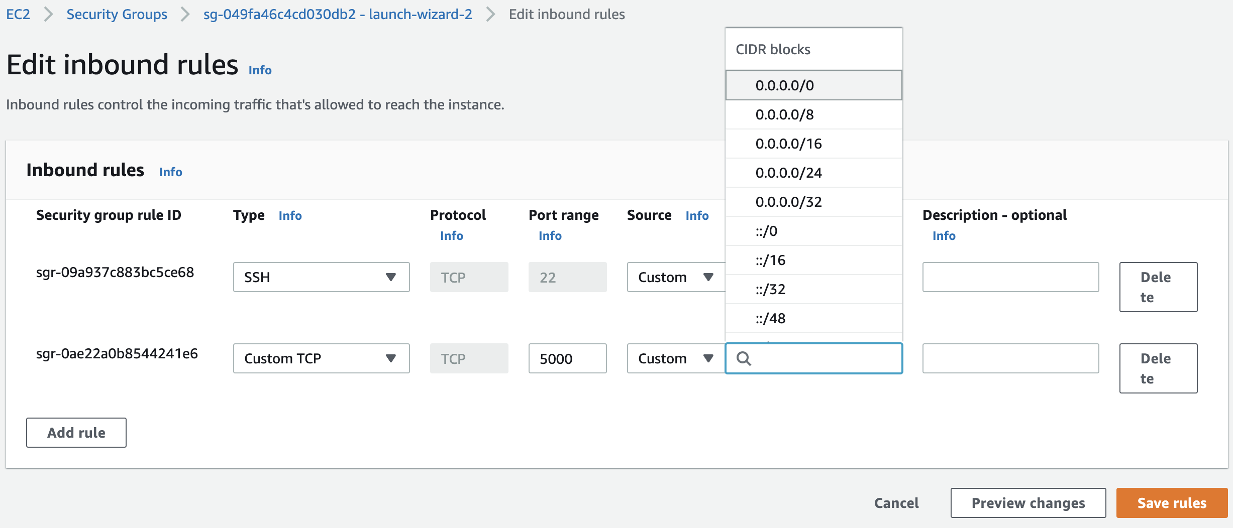
Fig. 82 Our instance should accept incoming SSH (port 22) and HTTP connections (port 5000). Specify CIDR blocks to specify the range of IP addresses that has access to the tracking server. Choosing 0.0.0.0/0 allows all incoming HTTP access.#
PostgreSQL DB#
Create database in the RDS console:
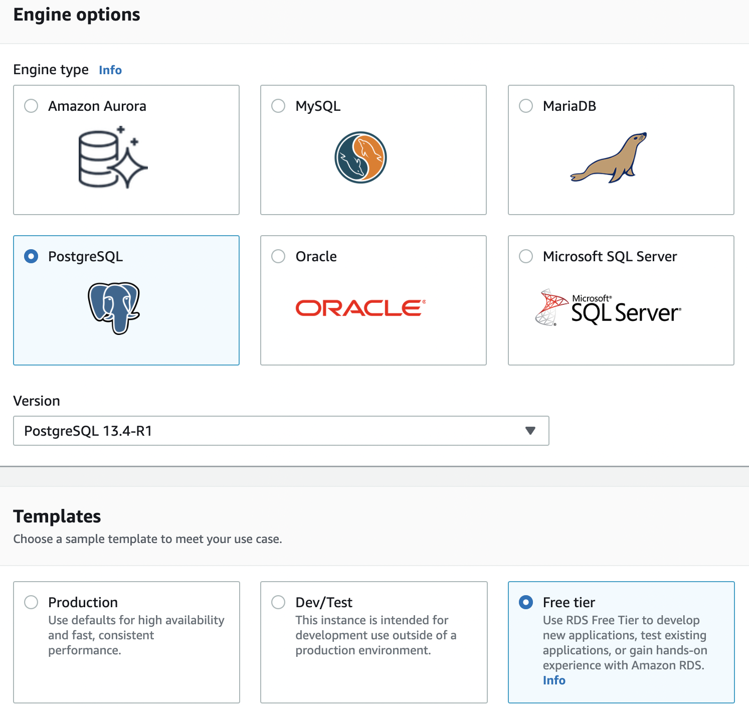
Fig. 83 Choosing an engine and template.#
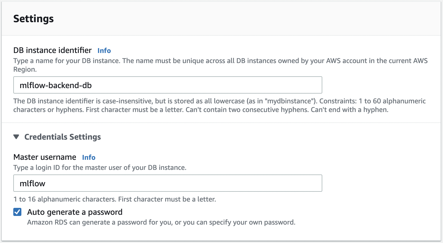
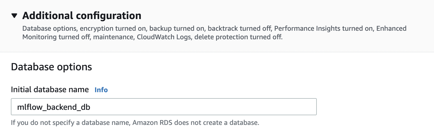
Fig. 84 Choosing identifier, and other names. Save master username, password, and initial database name. This will be used later. On the RDS dashboard, click on the database and look at “Connectivity & Security”. Take note of the endpoint which you will find here.#
Select the VPC security group of the DB under the same tab. Click the security group ID, and edit inbound rules by adding a new rule that allows PostgreSQL connections on the port 5432 from the security group of the EC2 instance for the tracking server:
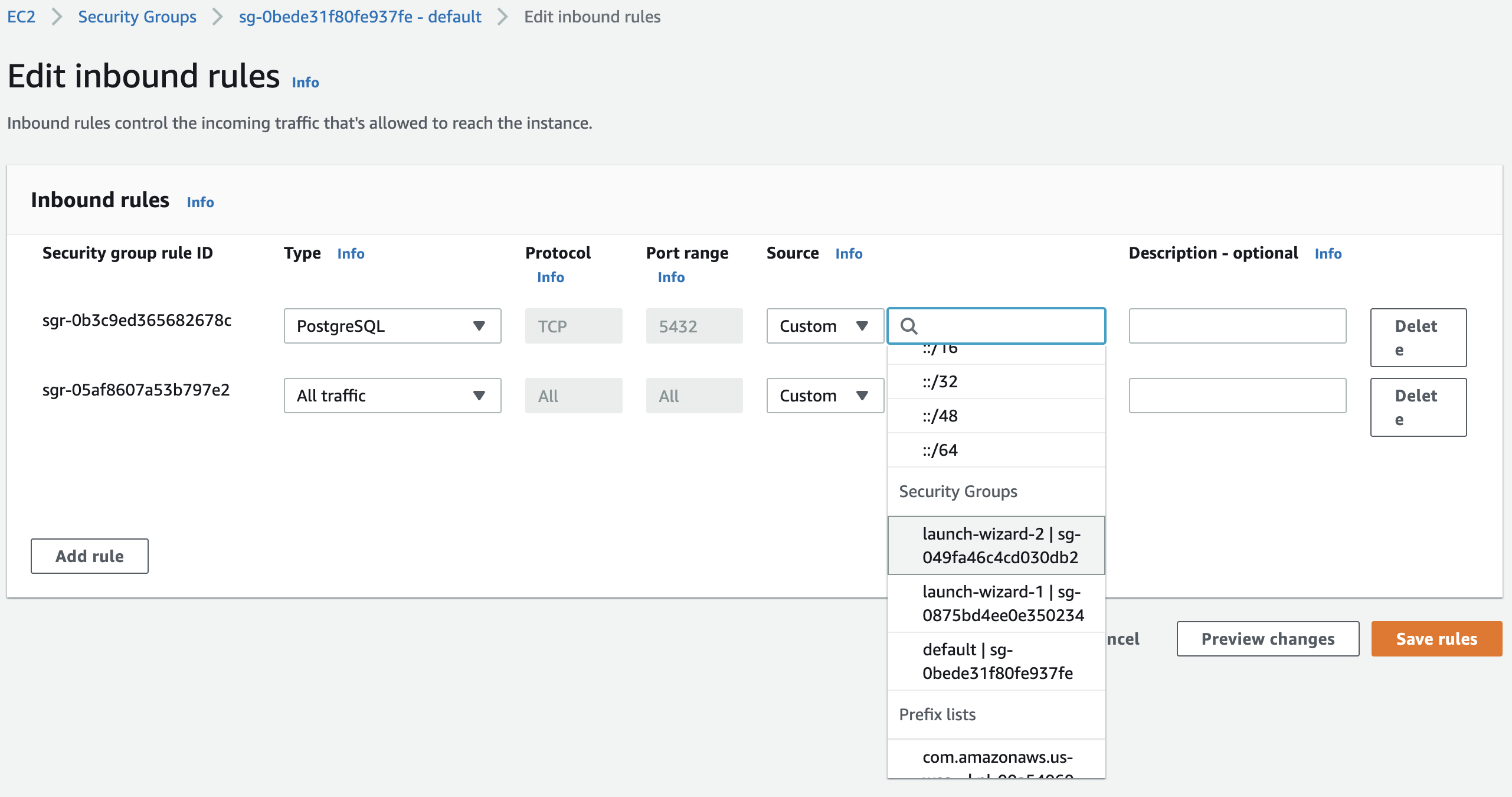
Fig. 85 Allow postgres connections from the tracking server to the backend database. Select the security group of the EC2 instance Fig. 82. This allows the tracking server to connect to the PostgreSQL database.#
Server config and launch#
Here we connect to the mlflow-tracking-server EC2 instance from our local terminal:
chmod 400 ~/.ssh/mlflow-tacking.pem
ssh -i "~/.ssh/mlflow-tracking.pem" ec2-user@ec2-34-209-62-152.us-west-2.compute.amazonaws.com
Run the following installation steps inside:
sudo yum update
pip3 install mlflow boto3 psycopg2-binary
aws configure
aws s3 ls       # Test
Running the server:
export DB_USER=mlflow
export DB_PASSWORD=ZbTddA0Zc8LxYcdLFUQr
export DB_ENDPOINT=mlflow-backend-database.csegt7oxppl.us-west-2.rds.amazonaws.com
export DB_NAME=mlflow_backend_database
export S3_BUCKET_NAME=mlflow-artifact-store-2

mlflow server -h 0.0.0.0 -p 5000 \
    --backend-store-uri=postgresql://${DB_USER}:${DB_PASSWORD}@${DB_ENDPOINT}:5432/${DB_NAME} \
    --default-artifact-root=s3://${S3_BUCKET_NAME}
Running a remote experiment#
Since we are allowed by the inbound rules to send information via HTTP to the tracking server, we should be able to send requests to it. Note that everything that follows is done in our local Jupyter notebook. After setting the tracking URI we should be able to manage experiments and the model registry through the client as before.
import mlflow
from mlflow.tracking import MlflowClient

TRACKING_SERVER_HOST = "ec2-34-209-62-152.us-west-2.compute.amazonaws.com"
mlflow.set_tracking_uri(f"http://{TRACKING_SERVER_HOST}:5000")
client = MlflowClient(tracking_uri=f"http://{TRACKING_SERVER_HOST}:5000")
Running an example experiment.
from sklearn.linear_model import LogisticRegression
from sklearn.datasets import load_iris
from sklearn.metrics import accuracy_score
from warnings import simplefilter
from sklearn.exceptions import ConvergenceWarning
simplefilter("ignore", category=ConvergenceWarning)


mlflow.set_experiment("iris")
X, y = load_iris(return_X_y=True)

for C in [10, 1, 0.1, 0.01, 0.001]:
    with mlflow.start_run(nested=True):
        params = {"C": C, "random_state": 42}
        lr = LogisticRegression(**params).fit(X, y)
        y_pred = lr.predict(X)

        mlflow.log_metric("accuracy", accuracy_score(y, y_pred))
        mlflow.log_params(params)
        mlflow.sklearn.log_model(lr, artifact_path="models")
2022/06/04 03:44:56 INFO mlflow.tracking.fluent: Experiment with name 'iris' does not exist. Creating a new experiment.
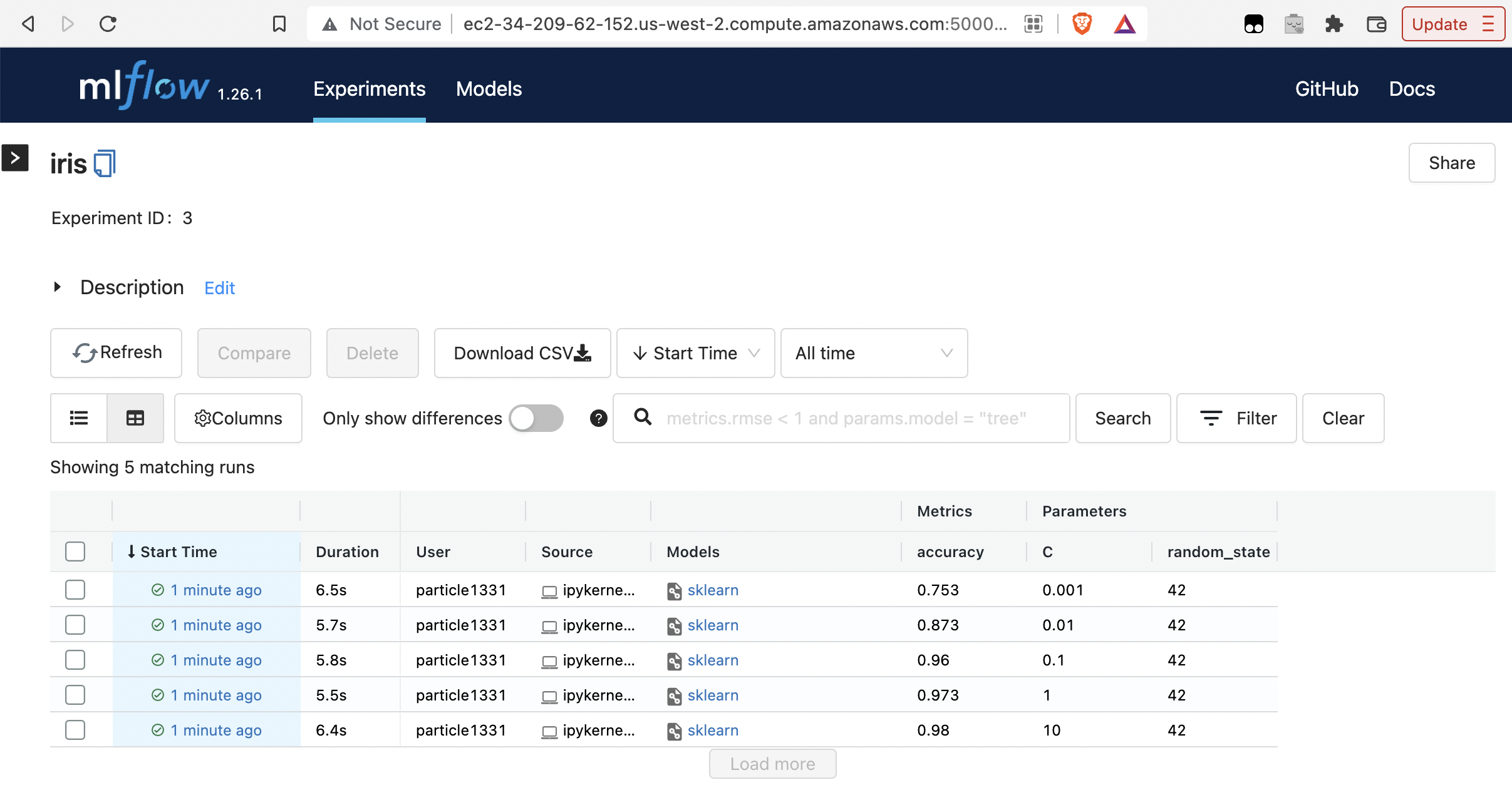
Fig. 86 Runs are recorded in the tracking UI.#
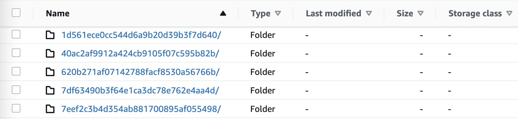
Fig. 87 We can see the runs artifacts stored in the S3 bucket.#