Backpropagation#


Readings: [Vie16] [AM16] [Wai18] [Kar22]
Introduction#
In this notebook, we introduce the backpropagation algorithm for efficient gradient computation on computational graphs. Backpropagation involves local message passing of activations in the forward pass, and gradients in the backward pass. The resulting time complexity is linear in the number of size of the network, i.e. the total number of weights and neurons for neural networks. Neural networks are computational graphs with nodes for differentiable operations. This fact allows scaling training large neural networks. We will implement a minimal scalar-valued autograd engine and a neural net library on top it to train a small regression model.
BP on computational graphs#
A neural network can be modelled as a directed acyclic graph (DAG) of nodes that implements a function \(f\), i.e. all computation flows from an input \(\boldsymbol{\mathsf{x}}\) to an output node \(f(\boldsymbol{\mathsf{x}})\) with no cycles. During training, this is extended to implement the calculation of the loss. Recall that our goal is to obtain parameter node values \(\hat{\boldsymbol{\Theta}}\) after optimization (e.g. with SGD) such that the \(f_{\hat{\boldsymbol{\Theta}}}\) minimizes the expected value of a loss function \(\ell.\) Backpropagation allows us to efficiently compute \(\nabla_{\boldsymbol{\Theta}} \ell\) for SGD after \((\boldsymbol{\mathsf{x}}, y) \in \mathcal{B}\) is passed to the input nodes.
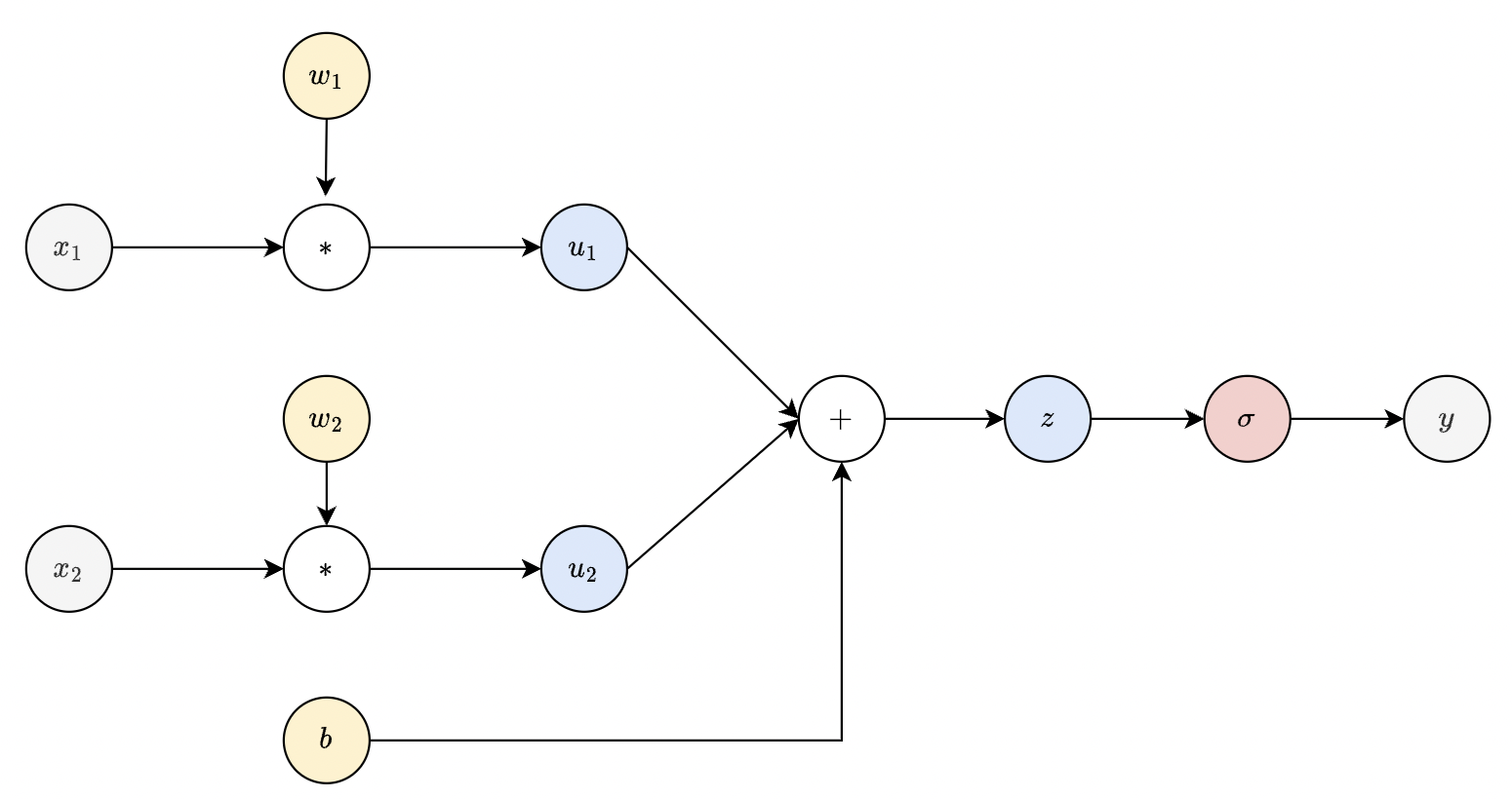
Fig. 29 Computational graph of a dense layer. Note that parameter nodes (yellow) always have zero fan-in.#
Forward pass. Forward pass computes \(f_{\boldsymbol{\Theta}}(\boldsymbol{\mathsf{x}}).\) All compute nodes are executed starting from the input nodes (which evaluates to the input vector \(\boldsymbol{\mathsf x}\)). This passed to its child nodes, and so on up to the loss node. The output value of each node is stored to avoid recomputation for child nodes that depend on the same node. This also preserves the network state for backward pass. Finally, forward pass builds the computational graph which is stored in memory. It follows that forward pass for one input is roughly \(O(E)\) in time and memory where \(E\) is the number of edges of the graph.
Backward pass. Backward computes gradients starting from the loss node \(\ell\) down to the input nodes \(\boldsymbol{\mathsf{x}}.\) The gradient of \(\ell\) with respect to itself is \(1\). This serves as the base step. For any other node \(u\) in the graph, we can assume that the global gradient \({\partial \ell}/{\partial v}\) is cached for each node \(v \in N_u\), where \(N_u\) are all nodes in the graph that depend on \(u\). On the other hand, the local gradient \({\partial v}/{\partial u}\) between adjacent nodes is specified analytically based on the functional dependence of \(v\) upon \(u.\) These are computed at runtime given current node values cached during forward pass.
The global gradient with respect to node \(u\) can then be inductively calculated using the chain rule: \(\frac{\partial \ell}{\partial u} = \sum_{v \in N_u} \frac{\partial \ell}{\partial v} \frac{\partial v}{\partial u}.\) This can be visualized as gradients flowing from the loss node to each network node. The flow of gradients will end on parameter and input nodes which depend on no other nodes. These are called leaf nodes. It follows that the algorithm terminates.

Fig. 30 Computing the global gradient for a single node. Note that gradient type is distinguished by color: local (red) and global (blue).#
This can be visualized as gradients flowing to each network node from the loss node. The flow of gradients will end on parameter and input nodes which have zero fan-in. Global gradients are stored in each compute node in the grad attribute for use by the next layer, along with node values obtained during forward pass which are used in local gradient computation. Memory can be released after the weights are updated. On the other hand, there is no need to store local gradients as these are computed as needed. Backward pass can be implemented roughly as follows:
class CompGraph:
    # ...

    def backward():
        for node in self.nodes():
            node.grad = None

        self.loss_node.grad = 1.0
        self.loss_node.backward()


class Node:
    # ...

    def backward(self):
        for parent in self.parents:
            parent.grad += self.grad * self.local_grad(parent)
            parent.degree -= 1
            if parent.degree == 0:
                parent.backward()
Each node has to wait for all incoming gradients from dependent nodes before passing the gradient to its parents. This is done by having a degree attribute that tracks whether all gradients from its dependent nodes have accumulated to a parent node. A newly created node starts with zero degree and is incremented each time a child node is created from it. In particular, the loss node has degree zero. Here self.grad is the global gradient which is equal to ∂L/∂(self) while the local gradient self.local_grad is equal to ∂(self)/∂(parent). So this checks out with the chain rule. See Fig. 31 below.
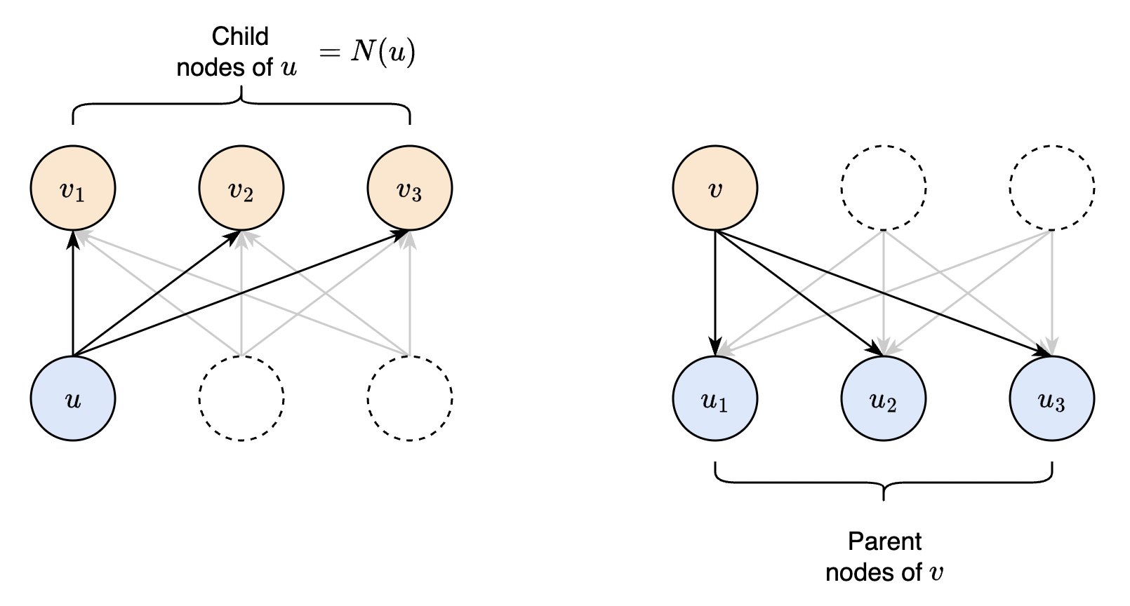
Fig. 31 Equivalent ways of computing the global gradient. On the left, the global gradient is computed by tracking the dependencies from \(u\) to each of its child node during forward pass. This is our formal statement before. Algorithmically, we start from each node in the upper layer. So instead, we contribute one term in the sum to each parent node. Eventually, all terms in the chain rule is accumulated and the parent node fires, sending gradients to its parent nodes in the next layer.#
Some characteristics of backprop which explains why it is ubiquitous in deep learning:
Modularity. Backprop is a useful tool for reasoning about gradient flow and can suggest ways to improve training or network design. Moreover, since it only requires local gradients between nodes, it allows modularity when designing deep neural networks. In other words, we can (in principle) arbitrarily connect layers of computation.
Runtime. Each edge is the DAG is passed exactly once (Fig. 31). Hence, the time complexity for finding global gradients is \(O(n_\mathsf{E})\) where \(n_\mathsf{E}\) is the number of edges in the graph, where we assume that each compute node and local gradient evaluation is constant time. For fully-connected networks, \(n_\mathsf{E} = n_\mathsf{M} + n_\mathsf{V}\) where \(n_\mathsf{M}\) is the number of weights and \(n_\mathsf{V}\) is the number of activations. It follows that one backward pass for an instance is proportional to the network size.
Memory. Each training step naively requires \(O(2 n_\mathsf{E})\) memory since we store both gradients and values. This can be improved by releasing the gradients and activations of non-leaf nodes in the previous layer once a layer finishes computing its gradient.
GPU parallelism. Note that forward computation can generally be parallelized in the batch dimension and often times in the layer dimension. This can leverage massive parallelism in the GPU significantly decreasing runtime by trading off memory. The same is true for backward pass which can also be expressed in terms of matrix multiplications! (3)
Creating and training a neural net from scratch#
Recall that all operations must be defined with specific local gradient computation for BP to work. In this section, we will implement a minimal autograd engine for creating computational graphs. This starts with the base Node class which has a data attribute for storing output and a grad attribute for storing the global gradient. The base class defines a backward method to solve for grad as described above.
import math
import random
random.seed(42)

from typing import final


class Node:
    def __init__(self, data, parents=()):
        self.data = data
        self.grad = 0             # ∂(loss)/∂(self)
        self._degree = 0          # no. of children
        self._parents = parents   # terminal node

    @final
    def backward(self):
        """Send global grads backward to parent nodes."""
        for parent in self._parents:
            parent.grad += self.grad * self._local_grad(parent)
            parent._degree -= 1
            if parent._degree == 0:
                parent.backward()

    def _local_grad(self, parent) -> float:
        """Compute local grads ∂(self)/∂(parent)."""
        raise NotImplementedError("Base node has no parents.")

    def __add__(self, other):
        self._degree += 1
        other._degree += 1
        return BinaryOpNode(self, other, op='+')

    def __mul__(self, other):
        self._degree += 1
        other._degree += 1
        return BinaryOpNode(self, other, op='*')

    def __pow__(self, n):
        assert isinstance(n, (int, float)) and n != 1
        self._degree += 1
        return PowOp(self, n)

    def relu(self):
        self._degree += 1
        return ReLUNode(self)

    def tanh(self):
        self._degree += 1
        return TanhNode(self)

    def __neg__(self):
        return self * Node(-1)

    def __sub__(self, other):
        return self + (-other)
Observe that only a handful of operations are needed to implement a fully-connected neural net:
class BinaryOpNode(Node):
    def __init__(self, x, y, op: str):
        """Binary operation between two nodes."""
        ops = {
            '+': lambda x, y: x + y,
            '*': lambda x, y: x * y
        }
        self._op = op
        super().__init__(ops[op](x.data, y.data), (x, y))

    def _local_grad(self, parent):
        if self._op == '+':
            return 1.0

        elif self._op == '*':
            i = self._parents.index(parent)
            coparent = self._parents[1 - i]
            return coparent.data

    def __repr__(self):
        return self._op


class ReLUNode(Node):
    def __init__(self, x):
        data = x.data * int(x.data > 0.0)
        super().__init__(data, (x,))

    def _local_grad(self, parent):
        return float(parent.data > 0)

    def __repr__(self):
        return 'relu'


class TanhNode(Node):
    def __init__(self, x):
        data = math.tanh(x.data)
        super().__init__(data, (x,))

    def _local_grad(self, parent):
        return 1 - self.data**2

    def __repr__(self):
        return 'tanh'


class PowOp(Node):
    def __init__(self, x, n):
        self.n = n
        data = x.data ** self.n
        super().__init__(data, (x,))

    def _local_grad(self, parent):
        return self.n * parent.data ** (self.n - 1)

    def __repr__(self):
        return f"** {self.n}"
Graph vizualization#
The next two functions help to visualize networks. The trace function just walks backward into the graph to collect all nodes and edges. This is used by the draw_graph which first draws all nodes, then draws all edges. For compute nodes we add a small juncture node which contains the name of the operation.
Show code cell source
# https://github.com/karpathy/micrograd/blob/master/trace_graph.ipynb
from graphviz import Digraph

def trace(root):
    """Builds a set of all nodes and edges in a graph."""

    nodes, edges = set(), set()

    def build(v):
        if v not in nodes:
            nodes.add(v)
            for child in v._parents:
                edges.add((child, v))
                build(child)

    build(root)
    return nodes, edges


def draw_graph(root):
    """Build diagram of computational graph."""

    dot = Digraph(format='svg', graph_attr={'rankdir': 'LR'}) # LR = left to right
    nodes, edges = trace(root)
    for n in nodes:

        # Add node to graph
        uid = str(id(n))
        dot.node(name=uid, label=f"data={n.data:.3f} | grad={n.grad:.4f} | deg={n._degree}", shape='record')

        # Connect node to op node if operation
        # e.g. if (5) = (2) + (3), then draw (5) as (+) -> (5).
        if len(n._parents) > 0:
            dot.node(name=uid+str(n), label=str(n))
            dot.edge(uid+str(n), uid)

    for child, v in edges:
        # Connect child to the op node of v
        dot.edge(str(id(child)), str(id(v)) + str(v))

    return dot
Creating graph for a dense unit. Observe that x1 has a degree of 2 since it has two children.
w1 = Node(-1.0)
w2 = Node(2.0)
b  = Node(4.0)
x  = Node(2.0)
t  = Node(3.0)

z = w1 * x + w2 * x + b
y = z.relu()
draw_graph(y)

Backward pass can be done by setting the initial gradient of the final node, then calling backward on it. Recall for the loss node loss.grad = 1.0. Observe that all gradients check out. Also, all degrees are zero, which means we did not overshoot the updates. This also means we can’t execute .backward() twice.
y.grad = 1.0
y.backward()
draw_graph(y)

Neural network#
Here we construct the neural network module. The Module class defines an abstract class that maintains a list of the parameters used in forward pass implemented in __call__. The decorator @final is to prevent any inheriting class from overriding the methods as doing so would result in a warning (or an error with a type checker).
from abc import ABC, abstractmethod

class Module(ABC):
    def __init__(self):
        self._parameters = []

    @final
    def parameters(self) -> list:
        return self._parameters

    @abstractmethod
    def __call__(self, x: list):
        pass

    @final
    def zero_grad(self):
        for p in self.parameters():
            p.grad = 0
The _parameters attribute is defined so that the parameter list is not constructed at each call of the parameters() method. Implementing layers from neurons:
import numpy as np
np.random.seed(42)


class Neuron(Module):
    def __init__(self, n_in, nonlinear=True, activation='relu'):
        self.n_in = n_in
        self.act = activation
        self.nonlin = nonlinear

        self.w = [Node(random.random()) for _ in range(n_in)]
        self.b = Node(0.0)
        self._parameters = self.w + [self.b]

    def __call__(self, x: list):
        assert len(x) == self.n_in
        out = sum((x[j] * self.w[j] for j in range(self.n_in)), start=self.b)
        if self.nonlin:
            if self.act == 'tanh':
                out = out.tanh()
            elif self.act == 'relu':
                out = out.relu()
            else:
                raise NotImplementedError("Activation not supported.")
        return out

    def __repr__(self):
        return f"{self.act if self.nonlin else 'linear'}({len(self.w)})"


class Layer(Module):
    def __init__(self, n_in, n_out, *args):
        self.neurons = [Neuron(n_in, *args) for _ in range(n_out)]
        self._parameters = [p for n in self.neurons for p in n.parameters()]

    def __call__(self, x: list):
        out = [n(x) for n in self.neurons]
        return out[0] if len(out) == 1 else out

    def __repr__(self):
        return f"Layer[{', '.join(str(n) for n in self.neurons)}]"


class MLP(Module):
    def __init__(self, n_in, n_outs, activation='relu'):
        sizes = [n_in] + n_outs
        self.layers = [Layer(sizes[i], sizes[i+1], i < len(n_outs)-1, activation) for i in range(len(n_outs))]
        self._parameters = [p for layer in self.layers for p in layer.parameters()]

    def __call__(self, x):
        for layer in self.layers:
            x = layer(x)
        return x

    def __repr__(self):
        return f"MLP[{', '.join(str(layer) for layer in self.layers)}]"
Testing model init and model call. Note that final node has no activation:
model = MLP(n_in=1, n_outs=[2, 2, 1])
print(model)
x = Node(1.0)
pred = model([x])
print(pred.data)
MLP[Layer[relu(1), relu(1)], Layer[relu(2), relu(2)], Layer[linear(2)]]
0.20429304314825944
draw_graph(pred)

Benchmarking#
Recall BP has time and memory complexity that is linear in the network size. This assumes each node executes in constant time and the outputs are stored. Moreover, the gradient should never be asymptotically slower than the function (assuming local gradient computation takes constant time). Testing this here empirically.
Show code cell source
from tqdm.notebook import tqdm
import time
import matplotlib.pyplot as plt
from matplotlib_inline import backend_inline
backend_inline.set_matplotlib_formats('svg')


x = [Node(1.0)] * 3
network_size  = []
fwd_times = {}
bwd_times = {}

for i in tqdm(range(15)):
    nouts = [200] * (i + 1) + [1]
    model = MLP(n_in=3, n_outs=nouts)

    fwd_times[i] = []
    bwd_times[i] = []

    for j in range(5):
        start = time.process_time()
        pred = model(x)
        end = time.process_time()
        fwd_times[i].append(end - start)

        pred.grad = 1.0
        start = time.process_time()
        pred.backward()
        end = time.process_time()
        bwd_times[i].append(end - start)

    network_size.append(len(model.parameters()) + sum(nouts) + 3)


for i, size in enumerate(network_size):
    for j in range(5):
        if j == 4 and i == len(network_size) - 1:
            plt.scatter(size, fwd_times[i][j], color="C0", edgecolor="black", s=15, label="forward")
            plt.scatter(size, bwd_times[i][j], color="C1", edgecolor="black", s=15, label="backward")
        else:
            plt.scatter(size, fwd_times[i][j], color="C0", edgecolor="black", s=15)
            plt.scatter(size, bwd_times[i][j], color="C1", edgecolor="black", s=15)

plt.legend()
plt.xlabel("n hidden")
plt.ticklabel_format(axis="x", style="sci", scilimits=(3, 3))
plt.grid(linestyle="dotted")

Figure. Roughly linear time complexity in network size for both forward and backward passes.
Training the network!#
Dataset. Our task is to learn from noisy data points around a true curve:
N = 500
X = np.linspace(-1, 5, N)
Y_true = X ** 2
Y = Y_true + 0.5 * np.random.normal(size=N)
Show code cell source
plt.figure(figsize=(6, 4))
plt.scatter(X, Y, label='data', s=2, alpha=0.9)
plt.ylabel('y')
plt.xlabel('x')
plt.legend();

Data loader. Helper for loading the samples:
import random

class DataLoader:
    def __init__(self, dataset):
        """Iterate over a partition of the dataset."""
        self.dataset = [(Node(x), Node(y)) for x, y in dataset]

    def load(self):
        return random.sample(self.dataset, len(self.dataset))

    def __len__(self):
        return len(self.dataset)
Model training. The function optim_step implements one step of SGD with batch size 1. Here loss_fn just computes the MSE between two nodes.
def optim_step(model, eps):
    for p in model.parameters():
        p.data -= eps * p.grad

def loss_fn(y_pred, y_true):
    return (y_pred - y_true) ** 2
Running the training algorithm:
def train(model, dataset, epochs):
    dataloader = DataLoader(dataset)
    history = []
    for _ in tqdm(range(epochs)):
        for x, y in dataloader.load():
            loss = loss_fn(model([x]), y)
            loss.grad = 1.0
            loss.backward()
            optim_step(model, eps=0.0001)

            model.zero_grad()
            history.append(loss.data)

    return history

dataset = list(zip(X, Y))
model = MLP(1, [8, 4, 1], 'tanh')
losses = train(model, dataset, epochs=1000)
Loss curve becomes more stable as we train futher:
Show code cell source
window = 5
loss_avg = []
for i in range(1, len(losses)):
    loss_avg.append(np.mean(losses[max(0, i - window):i]))

plt.plot(loss_avg)
plt.ylabel("loss (avg)")
plt.xlabel("steps")
plt.ylim(0, 100);

Model learned: ヾ( ˃ᴗ˂ )◞ • *✰
Show code cell source
plt.figure(figsize=(6, 4))
plt.scatter(X, Y, label='data', s=2, alpha=0.9)
plt.plot(X, [model([Node(_)]).data for _ in X], label='model', color='C1', linewidth=2)

plt.ylabel('y')
plt.xlabel('x')
plt.grid(linestyle="dotted")
plt.legend();

Appendix: Testing with autograd#
The autograd package allows automatic differentiation by building computational graphs on the fly every time we pass data through our model. Autograd tracks which data combined through which operations to produce the output. This allows us to take derivatives over ordinary imperative code. This functionality is consistent with the memory and time requirements outlined above for BP.
Scalars. Here we calculate \(\mathsf{y} = \boldsymbol{\mathsf x}^\top \boldsymbol{\mathsf x} = \sum_i {\boldsymbol{\mathsf{x}}_i}^2\) where the initialized tensor \(\boldsymbol{\mathsf{x}}\) initially has no gradient (i.e. None). Calling backward on \(\mathsf{y}\) results in gradients being stored on the leaf tensor \(\boldsymbol{\mathsf{x}}.\) Note that unlike our implementation, there is no need to set y.grad = 1.0. Moreover, doing so would result in an error as \(\mathsf{y}\) is not a leaf node in the graph.
import torch
import torch.nn.functional as F
print(torch.__version__)
2.0.0
x = torch.arange(4, dtype=torch.float, requires_grad=True)
print(x.grad)

y = x.reshape(1, -1) @ x
y.backward()
print((x.grad == 2*x).all().item())
None
True
Vectors. Let \(\boldsymbol{\mathsf y} = g(\boldsymbol{\mathsf x})\) and let \(\boldsymbol{{\mathsf v}}\) be a vector having the same length as \(\boldsymbol{\mathsf y}.\) Then y.backward(v) calculates
\(\sum_i {\boldsymbol{\mathsf v}}_i \frac{\partial {\boldsymbol{\mathsf y}}_i}{\partial {\boldsymbol{\mathsf x}}_j}\)
resulting in a vector of same length as \(\boldsymbol{\mathsf{x}}\) stored in x.grad. Note that the terms on the right are the local gradients. Setting \({\boldsymbol{\mathsf v}} = \frac{\partial \mathcal{L} }{\partial \boldsymbol{\mathsf y}}\) gives us the vector \(\frac{\partial \mathcal{L} }{\partial \boldsymbol{\mathsf x}}.\) Below \(\boldsymbol{\mathsf y}(\boldsymbol{\mathsf x}) = [x_0, x_1].\)
x = torch.rand(size=(4,), dtype=torch.float, requires_grad=True)
v = torch.rand(size=(2,), dtype=torch.float)
y = x[:2]

# Computing the Jacobian by hand
J = torch.tensor([
    [1, 0, 0, 0],
    [0, 1, 0, 0]], dtype=torch.float
)

# Confirming the above formula
y.backward(v)
(x.grad == v @ J).all()
tensor(True)
Remark. Gradient computation is not useful for tensors that is not part of backprop. Hence, we want to wrap our code in a torch.no_grad() context (or inside a function decorated with @torch.no_grad()) so that a computation graph is not built saving memory and compute. Note that the .detach() method returns a new tensor detached from the current graph but shares the same storage with the original one. In-place modifications on either tensor can result in subtle bugs.
Testing#
Finally, we write our tests with autograd to check the correctness of our implementation:
x = Node(-4.0)
z = Node(2) * x + Node(2) - x
q = z.relu() + z * x.tanh()
h = (z * z).relu()
y = (-h + q + q * x).tanh()
y.grad = 1.0
y.backward()

x_node, y_node, z_node = x, y, z
draw_graph(y_node)

x = torch.tensor(-4.0, requires_grad=True)
z = 2 * x + 2 - x
q = z.relu() + z * x.tanh()
h = (z * z).relu()
y = (-h + q + q * x).tanh()

z.retain_grad()
y.retain_grad()
y.backward()

x_torch, y_torch, z_torch = x, y, z

# forward
errors = []
errors.append(abs(x_node.data - x_torch.item()))
errors.append(abs(y_node.data - y_torch.item()))
errors.append(abs(z_node.data - z_torch.item()))

# backward
errors.append(abs(x_node.grad - x_torch.grad.item()))
errors.append(abs(y_node.grad - y_torch.grad.item()))
errors.append(abs(z_node.grad - z_torch.grad.item()))

print(f"Max absolute error: {max(errors):.2e}")
Max absolute error: 7.48e-08
Appendix: BP equations for MLPs#
Closed-form expressions for input and output gradients is more efficient to compute since no explicit passing of gradients between nodes is performed. Moreover, such expressions allow us to see how to express it in terms of matrix operations which are computed in parallel. In this section, we derive BP equations specifically for MLPs. Recall that a dense layer with weights \(\boldsymbol{\mathsf{w}}_j \in \mathbb{R}^d\) and bias \({b}_j \in \mathbb{R}\) computes given an input \(\boldsymbol{\mathsf{x}} \in \mathbb{R}^d\) the following equations for \(j = 1, \ldots, h\) where \(h\) is the layer width:
Given global gradients \(\partial \ell / \partial y_j\) that flow into the layer, we compute the global gradients of the nodes \(\boldsymbol{\mathsf{z}}\), \(\boldsymbol{\mathsf{w}}\), \(\boldsymbol{\mathsf{b}}\), and \(\boldsymbol{\mathsf{x}}\) in the layer. As discussed above, this can be done by tracking backward dependencies in the computational graph (Fig. 32).

Fig. 32 Node dependencies in compute nodes of a fully connected layer. All nodes \(\boldsymbol{\mathsf{z}}_k\) depend on the node \(\boldsymbol{\mathsf{y}}_j.\)#
Note that there can be cross-dependencies for activations such as softmax. For typical activations \(\phi,\) the Jacobian \(\mathsf{J}^{\phi}_{kj} = \frac{\partial y_k}{\partial z_j}\) reduces to a diagonal matrix. Following backward dependencies for the compute nodes:
Note that the second equation uses the gradients calculated in the first equation. Next, we compute gradients for the weights:
Observe the dependence of the weight gradient on the input makes it sensitive to scaling. This can introduce an effective scalar factor to the learning rate that is specific to each input dimension, making SGD diverge at early stages of training. This motivates network input normalization and layer output normalization.
Batch computation#
Let \(B\) be the batch size. Processing a batch of inputs in parallel, in principle, creates a graph consisting of \(B\) copies of the original computational graph that share the same parameters. The outputs of these combine to form the loss node \(\mathcal{L} = \frac{1}{B}\sum_b \ell_b.\) For usual activations, \(\boldsymbol{\mathsf{J}}^\phi = \text{diag}(\phi^\prime(\boldsymbol{\mathsf{z}}))\). The output and input gradients can be written in the following matrix notation for fast computation:
These correspond to the equations above since there is no dependence across batch instances. Note that the stacked output tensors \(\boldsymbol{\mathsf{Z}}\) and \(\boldsymbol{\mathsf{Y}}\) have shape \((B, h)\) where \(h\) is the layer width and \(B\) is the batch size. The stacked input tensor \(\boldsymbol{\mathsf{X}}\) has shape \((B, d)\) where \(d\) is the input dimension. Finally, the weight tensor \(\boldsymbol{\mathsf{W}}\) has shape \((d, h).\) For the weights, the contribution of the entire batch have to be accumulated (Fig. 33):
Remark. One way to remember these equations is that the shapes must check out.

Fig. 33 Node dependencies for a weight node. The nodes \(\boldsymbol{\mathsf{z}}_{bj}\) depend on \(\boldsymbol{\mathsf{w}}_{ij}\) for \(b = 1, \ldots, B.\)#
Cross entropy#
In this section, we compute the gradient across the cross-entropy loss. This can be calculated using backpropagation, but we will derive it symbolically to get a closed-form formula. Recall that cross-entropy loss computes for logits \(\boldsymbol{\mathsf{s}}\):
Calculating the derivatives, we get
where \(\delta_{j}^y\) is the Kronecker delta. This makes sense: having output values in nodes that do not correspond to the true class only contributes to increasing the loss. This effect is particularly strong when the model is confidently wrong such that \(p_y \approx 0\) on the true class and \(p_{j^*} \approx 1\) where \(j^* = \text{arg max}_j\, s_j\) is the predicted wrong class. On the other hand, increasing values in the node for the true class results in decreasing loss for all nodes. In this case, \(\text{softmax}(\boldsymbol{\mathsf{s}}) \approx \mathbf{1}_y,\) and \({\partial \ell}/{\partial \boldsymbol{\mathsf{s}}}\) becomes close to the zero vector, so that \(\nabla_{\boldsymbol{\Theta}} \ell\) is also close to zero.
The gradient of the logits \({\boldsymbol{\mathsf{S}}}\) can be written in matrix form where \(\mathcal{L} = \frac{1}{B}\sum_b \ell_b\):
Remark. Examples with similar features but different labels can contribute to a smoothing between the labels of the predicted probability vector. This is nice since we can use the probability value as a measure of confidence. We should also expect a noisy loss curve in the presence of significant label noise.
Gradient checking#
Computing the cross-entropy for a batch:
B = 32
N = 27

# forward pass
t = torch.randint(low=0, high=N, size=(B,))
x = torch.randn(B, 128, requires_grad=True)
w = torch.randn(128, N, requires_grad=True)
b = torch.randn(N,      requires_grad=True)
z = x @ w + b
y = torch.tanh(z)

for node in [x, w, b, z, y]:
    node.retain_grad()

# backprop batch loss
loss = -torch.log(F.softmax(y, dim=1)[range(B), t]).sum() / B
loss.backward()
Plotting the gradient of the logits:
fig, ax = plt.subplots(1, 2, figsize=(12, 6))
c = ax[0].imshow(y.grad.detach().numpy() * B, cmap='gray')
ax[1].imshow(-F.one_hot(t, num_classes=N).detach().numpy(), cmap='gray')
ax[0].set_ylabel("$B$")
ax[1].set_ylabel("$B$")
ax[0].set_xlabel("$N$")
ax[1].set_xlabel("$N$")
plt.colorbar(c, ax=ax[0])
fig.tight_layout();

Figure. Gradient of the logits for given batch (left) and actual targets (right). Notice the sharp contribution to decreasing loss by increasing the logit of the correct class. Other nodes contribute to increasing the loss. It’s hard to see, but incorrect pixels have positive values that sum to the pixel value in the target. Checking this to ensure correctness:
y.grad.sum(dim=1, keepdim=True).abs().mean()
tensor(2.0609e-09)
Recall that the above equations were vectorized with the convention that the gradient with respect to a tensor \(\boldsymbol{\mathsf{v}}\) has the same shape as \(\boldsymbol{\mathsf{v}}.\) In PyTorch, v.grad is the global gradient with respect to v of the tensor that called .backward() (i.e. loss in our case). The following computation should give us an intuition of how gradients flow backwards through the neural net starting from the loss to all intermediate results:
J = 1 - y**2                                    # Jacobian
δ_tk = F.one_hot(t, num_classes=N)              # Kronecker delta
dy = - (1 / B) * (δ_tk - F.softmax(y, dim=1))   # logits grad
dz = dy * J
dx = dz @ w.T
dw = x.T @ dz
db = dz.sum(0, keepdim=True)
Refer to (7), (3), (4), (5), and (6) above. These equations can be checked using autograd as follows:
def compare(name, dt, t):
    exact  = torch.all(dt == t.grad).item()
    approx = torch.allclose(dt, t.grad, rtol=1e-5)
    maxdiff = (dt - t.grad).abs().max().item()
    print(f'{name:<3s} | exact: {str(exact):5s} | approx: {str(approx):5s} | maxdiff: {maxdiff:.2e}')


compare('y', dy, y)
compare('z', dz, z)
compare('x', dx, x)
compare('w', dw, w)
compare('b', db, b)
y   | exact: False | approx: True  | maxdiff: 1.86e-09
z   | exact: False | approx: True  | maxdiff: 1.16e-10
x   | exact: False | approx: True  | maxdiff: 1.86e-09
w   | exact: False | approx: True  | maxdiff: 1.86e-09
b   | exact: False | approx: True  | maxdiff: 2.33e-10
■