Activations and Gradients

---

Readings: [BKH16] [IS15]

Introduction

Training neural nets involves computation across millions of weights and activations. Experience tells us that this process is fragile. In this notebook, we attach hooks in order to deep neural nets to analyze the statistics of activations and gradients during training, and consider pitfalls when they are improperly scaled. Finally, we introduce layer normalization (LN) [BKH16] which allows stable propagation of activations and gradients across layers. This makes training deep networks so much easier (e.g. without a lot of hyperparameter tuning).

In the appendix, we consider the effects of the choice of activation function on training dynamics. Deep MLPs suffer from rank collapse where the dimensionality of the output space of each layer degenerates with depth. We find empirically that batch normalization [IS15] avoids rank collapse in MLPs, while LN does not. This is consistent with theoretical results in [DKB+20] and [DCL21]. Finally, we introduce residual connections which forces the network to model residuals to the identity function and allow multiple paths for the gradient to flow to earlier layers. It will be shown that residual connections diminish rank collapse.

Preliminaries

import math
import torch
import random
import warnings
import numpy as np
import pandas as pd
import matplotlib.pyplot as plt
from pathlib import Path
from matplotlib_inline import backend_inline

DATASET_DIR = Path("./data").absolute()
RANDOM_SEED = 1
DEBUG = False
MATPLOTLIB_FORMAT = "png" if DEBUG else "svg"

def set_seed(s: int):
    random.seed(s)
    np.random.seed(s)
    torch.manual_seed(s)

set_seed(RANDOM_SEED)
warnings.simplefilter(action="ignore")
backend_inline.set_matplotlib_formats(MATPLOTLIB_FORMAT)

Still using the names dataset from the previous notebook:

import os
if not os.path.isfile("./data/surnames_freq_ge_100.csv"):
    !wget -O ./data/surnames_freq_ge_100.csv https://raw.githubusercontent.com/particle1331/spanish-names-surnames/master/surnames_freq_ge_100.csv
    !wget -O ./data/surnames_freq_ge_20_le_99.csv https://raw.githubusercontent.com/particle1331/spanish-names-surnames/master/surnames_freq_ge_20_le_99.csv
else:
    print("Data files already exist.")

col = ["surname", "frequency_first", "frequency_second", "frequency_both"]
df1 = pd.read_csv(DATASET_DIR / "surnames_freq_ge_100.csv", names=col, header=0)
df2 = pd.read_csv(DATASET_DIR / "surnames_freq_ge_20_le_99.csv", names=col, header=0)

Show code cell output Hide code cell output

Data files already exist.

FRAC_LIMIT = 0.10 if DEBUG else 1.0
df = pd.concat([df1, df2], axis=0)[["surname"]].sample(frac=FRAC_LIMIT)
df = df.reset_index(drop=True)
df["surname"] = df["surname"].map(lambda s: s.lower())
df["surname"] = df["surname"].map(lambda s: s.replace("de la", "dela"))
df["surname"] = df["surname"].map(lambda s: s.replace(" ", "_"))
df = df[["surname"]].dropna().astype(str)

names = [
    n for n in df.surname.tolist() 
    if ("'" not in n) and ('ç' not in n) and (len(n) >= 2)
]

for j in range(5):
    print(names[j])

agredano
poblador
girba
rabanales
yucra

Datasets

Defining here the dataset class used in the previous notebook:

import torch
from torch.utils.data import Dataset

class CharDataset(Dataset):
    def __init__(self, contexts: list[str], targets: list[str], chars: str):
        self.chars = chars
        self.ys = targets
        self.xs = contexts
        self.block_size = len(contexts[0])
        self.itos = {i: c for i, c in enumerate(self.chars)}
        self.stoi = {c: i for i, c in self.itos.items()}

    def get_vocab_size(self):
        return len(self.chars)
    
    def __len__(self):
        return len(self.xs)
    
    def __getitem__(self, idx):
        x = self.encode(self.xs[idx])
        y = torch.tensor(self.stoi[self.ys[idx]]).long()
        return x, y 
        
    def decode(self, x: torch.tensor) -> str:
        return "".join([self.itos[c.item()] for c in x])

    def encode(self, word: str) -> torch.tensor:
        return torch.tensor([self.stoi[c] for c in word]).long()


def build_dataset(names, block_size=3):
    """Build word context -> next char target lists from names."""
    xs = []     # context list
    ys = []     # target list
    for name in names:
        context = ["."] * block_size
        for c in name + ".":
            xs.append(context)
            ys.append(c)
            context = context[1:] + [c]
    
    chars = sorted(list(set("".join(ys))))
    return CharDataset(contexts=xs, targets=ys, chars=chars)

Example dataset with block size 3:

dataset = build_dataset(names, block_size=3)
xs = []
ys = []
for i in range(7):
    x, y = dataset[i]
    xs.append(x)
    ys.append(y)
    print("".join(dataset.decode(x)), "-->", dataset.itos[y.item()])

... --> a
..a --> g
.ag --> r
agr --> e
gre --> d
red --> a
eda --> n

Ideally, we should use a stratified k-fold that ensures character distribution is the same between splits. But too lazy. Here we just partition the names dataset by index to create the validation and train datasets.

SPLIT_RATIO = 0.30
split_point = int(SPLIT_RATIO * len(names))
names_train = names[:split_point]
names_valid = names[split_point:]
train_dataset = build_dataset(names_train, block_size=3)
valid_dataset = build_dataset(names_valid, block_size=3)

len(train_dataset), len(valid_dataset)

(186339, 433815)

Weight initialization

SGD requires choosing an arbitrary starting point \(\boldsymbol{\Theta}_{\text{init}}.\) Setting all weights to zero or some constant does not work as symmetry in the neurons of the network will make it difficult (if not impossible) to train the model. Hence, setting the weights randomly to break symmetry is a good starting point. However, this is still not enough since the variance of every neuron is additive (again due to symmetry and some assumptions):

\[{\sigma_{\boldsymbol{\mathsf{y}}}} = \sqrt{n} \cdot {\sigma_{\boldsymbol{\mathsf{w}}}} \, {\sigma_{\boldsymbol{\mathsf{x}}}}\]

where \(n = |\boldsymbol{\mathsf{x}}|.\)

import seaborn as sns

x = torch.randn(1000, 100)
w = torch.randn( 100, 200)
y = x @ w

Show code cell source Hide code cell source

plt.figure(figsize=(5, 3))
sns.distplot(x.reshape(-1), color="C0", label='$\mathbf{x}$ (input)');
sns.distplot(y.reshape(-1), color="C1", label='$\mathbf{y}$ (output)');
plt.legend();

Observe that the output \(\boldsymbol{\mathsf{y}} = \boldsymbol{\mathsf{x}}^\top \boldsymbol{\mathsf{w}}\) for normally distributed \(\boldsymbol{\mathsf{x}}\) and \(\boldsymbol{\mathsf{w}}\) starts to spread out. This makes sense since we are adding \(n\) terms where where \(n = |\boldsymbol{\mathsf{x}}|.\) Ideally, we want \(\boldsymbol{\mathsf{y}}\) to have the same standard deviation to maintain stable activation flow. Otherwise, activations will recursively grow at each layer. This becomes increasingly problematic with depth.

Dead neurons. Activations have regions where their gradients saturate, so it is very important to control the range of preactivations. A dead neuron has vanishingly small gradients for most training examples. This means that the weights for this neuron will change very slowly compared to other neurons.

A neuron can be dead at initialization or die in the course of training. For instance, a high learning rate can result in large weights that saturate the neurons similar to the situation above. For dense layers, dead neurons tend to remain dead for a long time since weight gradients are too small to significantly change the existing weights for that neuron.

Show code cell source Hide code cell source

activations = {
    "tanh": torch.tanh,
    "relu": torch.relu,
}

def d(f, x):
    """Compute derivative of activation with respect to x."""
    y = f(x)
    y.backward(torch.ones_like(x))
    return x.grad

def plot_activation(act: str, ax, x):
    x.grad = None
    f = activations[act]
    y = f(x)
    df = d(f, x)
    x, y = x.detach().numpy(), y.detach().numpy()
    
    # Plotting
    ax.plot(x, y,  linewidth=2, color='red',   label="f(x)")
    ax.plot(x, df, linewidth=2, color='black', label="f'(x)")
    ax.set_title(act)
    ax.grid(linestyle="dashed")
    ax.set_ylim(-1.5, 4)
    if act == "tanh":
        ax.axvspan(-5, -1.8183, -10, 10, color='lightgray')
        ax.axvspan(1.8183, 5,   -10, 10, color='lightgray')
    elif act == "relu":
        ax.axvspan(-5, 0, -10, 10, color='lightgray', label="|f'(x)| ≤ 0.1")
        ax.legend(loc='lower right')
    

# Plotting
fig, ax = plt.subplots(1, 2, figsize=(10, 3.5))

x = torch.linspace(-5, 5, 1000, requires_grad=True)
for i, act_name in enumerate(activations.keys()):
    plot_activation(act_name, ax[i], x)  # divmod(m, n) = m // n, m % n

fig.tight_layout()

Figure. Plotting activations and activation gradients. Saturation regions where derivatives are small (here set to 0.1) are highlighted gray.

Xavier init. [GB10] Since the \(\sigma_{\boldsymbol{\mathsf{y}}} = \sqrt{n} \cdot \sigma_{\boldsymbol{\mathsf{w}}} \, \sigma_{\boldsymbol{\mathsf{x}}}\), one straightforward fix is to initialize the weights \(\boldsymbol{\mathsf{w}}\) with a distribution having \({\sigma_{\boldsymbol{\mathsf{w}}}}=\frac{1}{\sqrt{n}}\) where \(n = |\boldsymbol{\mathsf{x}}|.\) Moreover, we set biases to zero. Note that setting the standard deviation turns out to be equivalent to just scaling the random variable with \(\frac{1}{\sqrt{n}}\) by linearity of expectation:

x = torch.randn(1000, 100)
w = torch.randn( 100, 200)  # Xavier normal. For xavier uniform, set w ~ U[-a, a] with a = (3 / n) ** 0.5
y = x @ (w / np.sqrt(100))

Show code cell source Hide code cell source

plt.figure(figsize=(5, 3))
sns.distplot(x.reshape(-1), color="C0", label='$\mathbf{x}$ (input)')
sns.distplot(y.reshape(-1), color="C1", label='$\mathbf{y}$ (output)')
plt.ylim(0, 0.6)
plt.legend();

Remark. For dense layers, the BP equation that relates input and output gradients is linear with \(\boldsymbol{\mathsf{w}}^\top.\) Improper scaling of weights can therefore cause vanishing or exploding gradients for MLPs at initialization, i.e. recursive multiplication of random weight matrices can increase or decrease gradients exponentially with depth. Hence, we can alternatively sample weights with \(\sigma_{\boldsymbol{\mathsf{w}}} = \frac{1} {\sqrt{n_\text{out}}}.\) Indeed, weight initialization is sometimes implemented with fan-average mode:

\[\sigma_{\boldsymbol{\mathsf{w}}} = \sqrt{\frac{2}{{n_\text{in} + n_\text{out}}}}.\]

Gain. Note that this scale factor only holds for linear layers. Nonlinear activations squashes its input which compounds as we stack layers in deep networks. The factor \(\mathsf{g}\) such that \({\sigma_{\boldsymbol{\mathsf{y}}}} = \mathsf{g} \cdot {\sigma_{\boldsymbol{\mathsf{x}}}}\) in called gain. This can be introduced as a factor on the standard deviation of the weights, i.e. setting the parameters of the distribution such that \(\sigma_{\boldsymbol{\mathsf{w}}} = \mathsf{g} \frac{1}{\sqrt{n}}\) where \(n = |\boldsymbol{\mathsf{x}}|\) for some \(\mathsf{g} > 0.\) Typically, weights are sampled from either normal or uniform distributions.

Show code cell source Hide code cell source

fig, ax = plt.subplots(1, 2, figsize=(8, 3))

n = 100
x = torch.randn(1000, n)
z = torch.tanh(x)   # Note: input of a hidden layer is an activation
w = torch.randn(n, 200) / n ** 0.5
y = z @ w

sns.distplot(x.reshape(-1), ax=ax[0], color="C0", label='$\mathbf{x}$ (input)');
sns.distplot(y.reshape(-1), ax=ax[0], color="C1", label='$\mathbf{y}$ (output)');
ax[0].set_title(r"$w \sim N(0, \sigma^2),$ $\sigma = n ^{-0.5}$", size=12)
ax[0].set_ylim(0, 0.8)

g = 5 / 3   # tanh gain
x = torch.randn(1000, n)
z = torch.tanh(x)
w = torch.randn(n, 200) * g / n ** 0.5
y = z @ w

sns.distplot(x.reshape(-1), ax=ax[1], color="C0", label='$\mathbf{x}$ (input)');
sns.distplot(y.reshape(-1), ax=ax[1], color="C1", label='$\mathbf{y}$ (output)');

ax[1].set_title(r"$w \sim N(0, \sigma^2),$ $\sigma = \frac{5}{3} {n}^{-0.5}$", size=12)
ax[1].set_ylim(0, 0.8)
ax[1].legend()
fig.tight_layout();

Kaiming init. Note that \(\mathsf{g}\) for an activation is usually obtained using some heuristic or by performing empirical tests, e.g. [HZRS15b] sets \(\mathsf{g} = \sqrt{2}\) since half of ReLU outputs are zero in the calculation of variance (see proof). See also calculate_gain for other commonly used activations.

PyTorch default for nn.Linear is essentially \(\mathsf{g} = \frac{1}{\sqrt{3}}\) with Xavier uniform fan-in initialization. Note that the standard deviation of the uniform distribution \(U[-a, a]\) is specified by the bound \(a\), i.e. \(\sigma = \frac{a}{\sqrt{3}}.\) The Pytorch implementation sets \(a = \frac{1}{\sqrt{n}}\) getting an effective gain of \(\frac{1}{\sqrt{3}}.\)

import torch.nn as nn

fan_in = 100
lin = nn.Linear(fan_in, 1234)
w = lin.weight.data
w.std(), 1 / (np.sqrt(3) * np.sqrt(fan_in))

(tensor(0.0576), 0.05773502691896258)

Remark. The formula for \(\sigma\) of \(U[-a, a]\) also explains the form of nn.init.kaiming_uniform_.

Logits. Xavier initialization can also be applied to the logits layer. It essentially acts as softmax temperature:

import torch.nn.functional as F

x = torch.randn(1, 30)
w = torch.randn(30, 10)
y0 = F.softmax(x @ w)
y1 = F.softmax(x @ (w / np.sqrt(30)))

Show code cell source Hide code cell source

fig, ax = plt.subplots(1, 2, figsize=(8, 3))
ax[0].set_title(r"$\sigma = 1$", size=11)
ax[1].set_title(r"$\sigma = {1}/{\sqrt{30}}$", size=11)
ax[0].set_xlabel("class index")
ax[1].set_xlabel("class index")
ax[0].bar(range(10), y0[0])
ax[1].bar(range(10), y1[0]);

Training with hooks

In our experiments, we use total steps per run instead of epochs. The following class wraps a data loader so that the iterator resets whenever the number of steps exceed one epoch (i.e. whenever a single pass over the entire training dataset has been reached):

class InfiniteDataLoader:
    def __init__(self, data_loader):
        self.data_loader = data_loader
        self.data_iterator = iter(self.data_loader)

    def __iter__(self):
        return self

    def __next__(self):
        try:
            batch = next(self.data_iterator)
        except StopIteration:
            self.data_iterator = iter(self.data_loader)
            batch = next(self.data_iterator)
        return batch

The Trainer class below streamlines model training (see previously notebook). Note that the class is augmented with hooks which we will use to obtain activation and gradient statistics during forward and backward passes. The hooks are attached to the model before training, then removed after. We skip validation during training since our current concern is training dynamics (not generalization).

from tqdm.notebook import tqdm
from contextlib import contextmanager
from torch.utils.data import DataLoader

DEVICE = "mps"


@contextmanager
def eval_context(model):
    """Temporarily set to eval mode inside context."""
    state = model.training
    model.eval()
    try:
        yield
    finally:
        model.train(state)


class Trainer:
    def __init__(self,
                 model, optim, loss_fn, 
                 scheduler=None,
                 callbacks=[],
                 device=DEVICE, verbose=True):
        
        self.model = model
        self.optim = optim
        self.device = device
        self.loss_fn = loss_fn
        self.logs = {"train": {"loss": []}}
        self.verbose = verbose
        self.scheduler = scheduler
        self.callbacks = callbacks
        self.forward_hooks = []
        self.backward_hooks = []
    
    def __call__(self, x):
        return self.model(x.to(self.device))

    def forward(self, batch):
        x, y = batch
        x = x.to(self.device)
        y = y.to(self.device)
        return self.model(x), y

    def train_step(self, batch):
        preds, y = self.forward(batch)
        loss = self.loss_fn(preds, y)
        loss.backward()
        self.optim.step()
        self.optim.zero_grad()
        return loss

    @torch.inference_mode()
    def valid_step(self, batch):
        preds, y = self.forward(batch)
        loss = self.loss_fn(preds, y, reduction="sum")
        return loss

    def register_hooks(self,            # !!!
                       fwd_hooks=[], 
                       bwd_hooks=[], 
                       layer_types=(nn.Linear, nn.Conv2d)):
        
        for _, module in self.model.named_modules():
            if isinstance(module, layer_types):
                for f in fwd_hooks:
                    h = module.register_forward_hook(f)
                    self.forward_hooks.append(h)
                
                for g in bwd_hooks:
                    h = module.register_backward_hook(g)
                    self.backward_hooks.append(h)

    def remove_hooks(self):
        for h in self.forward_hooks + self.backward_hooks:
            h.remove()
    
    def run(self, steps, train_loader):
        train_loader = InfiniteDataLoader(train_loader)
        for _ in tqdm(range(steps)):
            # optim and lr step
            batch = next(train_loader)
            loss = self.train_step(batch)
            if self.scheduler:
                self.scheduler.step()

            # step callbacks
            for callback in self.callbacks:
                callback()

            # logs @ train step
            self.logs["train"]["loss"].append(loss.item())

    def evaluate(self, data_loader):
        with eval_context(self.model):
            valid_loss = 0.0
            for batch in data_loader:
                loss = self.valid_step(batch)
                valid_loss += loss.item()

        return {"loss": valid_loss / len(data_loader.dataset)}

Forward hooks are expected to look like:

hook(module, input, output) -> None or modified output

On the other hand, backward hook functions should look like:

hook(module, grad_in, grad_out) -> None or modified grad_in

The following classes are for handling outputs of the hook functions:

class HookHandler:
    def __init__(self):
        self.records = {}

    def hook_fn(self, module, input, output):
        raise NotImplementedError


class OutputStats(HookHandler):
    def hook_fn(self, module, input, output):
        self.records[module] = self.records.get(module, [])
        self.records[module].append(output)


class WeightGradientStats(HookHandler):
    def hook_fn(self, module, grad_in, grad_out):
        self.records[module] = self.records.get(module, [])
        for t in grad_in:
            if t is not None and t.shape == module.weight.data.shape:
                self.records[module].append(t)


class ActivationGradientStats(HookHandler):
    def hook_fn(self, module, grad_in, grad_out):
        self.records[module] = self.records.get(module, [])
        for t in grad_in:
            if t is not None:
                self.records[module].append(grad_in[0])


class DyingReluStats(HookHandler):
    def __init__(self, sat_threshold=1e-8, frac_threshold=0.95):
        super().__init__()
        self.sat_threshold = sat_threshold
        self.frac_threshold = frac_threshold

    def hook_fn(self, module, input, output):
        self.records[module] = self.records.get(module, [])
        B = output.shape[0]
        count_dead = ((output < self.sat_threshold).float().sum(dim=0) / B) > self.frac_threshold
        frac_dead = count_dead.float().mean()
        self.records[module].append(frac_dead.item())

Setting up our experiment harness:

def get_model(vocab_size: int,
              block_size: int,
              emb_size: int,
              width: int,
              num_linear: int):

    layers = [
        nn.Embedding(vocab_size, emb_size), 
        nn.Flatten(),
        nn.Linear(block_size * emb_size, width), 
        nn.ReLU()
    ] 
    
    for _ in range(num_linear):
        layers.append(nn.Linear(width, width))
        layers.append(nn.ReLU())

    layers.append(nn.Linear(width, vocab_size))
    model = nn.Sequential(*layers)
    return model
    

def init_model(model, fn):
    """Expected `fn` modifies linear layer weights in-place. See 
    https://pytorch.org/docs/stable/nn.init.html for init functions."""
    for m in model.modules():
        if isinstance(m, nn.Linear):
            fn(m.weight)
            if m.bias is not None:
                nn.init.zeros_(m.bias)
        if isinstance(m, nn.Embedding):
            g = torch.Generator().manual_seed(RANDOM_SEED)
            nn.init.normal_(m.weight, generator=g)
    return model


def run(model,
        train_dataset: Dataset,
        batch_size: int,
        hooks: list[dict], 
        steps: int, 
        lr: float) -> Trainer:

    # Setup optimization and data loader
    set_seed(RANDOM_SEED)
    loss_fn = F.cross_entropy
    model = model.to(DEVICE)
    optim = torch.optim.SGD(model.parameters(), lr=lr)
    trainer = Trainer(model, optim, loss_fn, device=DEVICE)
    train_loader = DataLoader(train_dataset, batch_size=batch_size, drop_last=True, shuffle=True)

    # Finally, training...
    try:
        for hook_dict in hooks:
            trainer.register_hooks(
                fwd_hooks=[h.hook_fn for h in hook_dict["fwd_hooks"]], 
                bwd_hooks=[h.hook_fn for h in hook_dict["bwd_hooks"]], 
                layer_types=hook_dict["layer_types"]
            )

        trainer.run(steps=steps, train_loader=train_loader)

    except Exception as e:
        print(e)
    finally:
        trainer.remove_hooks()

    return trainer

The task and model used here is from the previous notebook. In the init_model function, we iterate over the layers and apply a function from the nn.init library to modify layer weights in-place. The xavier_uniform_ implementation uses fan average mode. This is applied to linear layer weights, while biases are set to zero. Finally, the embedding layer is initialized with weights from a Gaussian distribution.

def init_hooks() -> list[dict]:
    global dead_relu_stats
    global relu_outs_stats
    global relu_grad_stats
    global linear_outs_stats
    global linear_grad_stats

    dead_relu_stats = DyingReluStats(sat_threshold=1e-8, frac_threshold=0.95)
    relu_outs_stats = OutputStats()
    relu_grad_stats = ActivationGradientStats()
    linear_outs_stats = OutputStats()
    linear_grad_stats = WeightGradientStats()
    
    return [
        {
            "fwd_hooks": [linear_outs_stats], 
            "bwd_hooks": [linear_grad_stats], 
            "layer_types": (nn.Linear,)
        },
        {
            "fwd_hooks": [dead_relu_stats, relu_outs_stats], 
            "bwd_hooks": [relu_grad_stats], 
            "layer_types": (nn.ReLU,)
        }
    ]
    

model_params = {
    "vocab_size": 29,
    "block_size": 3,
    "emb_size": 10,
    "width": 30,
    "num_linear": 2
}

train_params = {
    "steps": 1000,
    "batch_size": 32,
    "lr": 0.1
}

g = lambda: torch.Generator().manual_seed(RANDOM_SEED)
init_fn = lambda w: nn.init.xavier_uniform_(w, gain=np.sqrt(2), generator=g())
model = init_model(get_model(**model_params), init_fn)
hooks = init_hooks()
trainer = run(model, train_dataset, **train_params, hooks=hooks)

Show code cell source Hide code cell source

def moving_avg(a, window=0.05):
    ma = []
    steps = len(a)
    w = int(window * steps)
    for s in range(steps):
        ma.append(np.mean(a[-w + s + 1: s + 1]))
    return ma

def plot_training_loss(trainer, window=0.05, figsize=(5, 3)):
    train_loss = trainer.logs["train"]["loss"]
    train_loss_ma = moving_avg(train_loss, window)

    plt.figure(figsize=figsize)
    plt.plot(trainer.logs["train"]["loss"], alpha=0.5, label="train")
    plt.plot(train_loss_ma, color="C0", label="train (MA)")
    plt.ylabel("loss")
    plt.xlabel("steps")
    plt.ylim(min(trainer.logs["train"]["loss"]) - 0.2, min(max(trainer.logs["train"]["loss"]) + 0.2, 5.0))
    plt.grid(linestyle="dotted", alpha=0.6)
    plt.legend();

plot_training_loss(trainer)

Histograms

The hooks stored activation and gradient statistics during training which we now visualize:

Colorful dimension

Show code cell source Hide code cell source

def plot_training_histograms(stats: list[HookHandler], 
                             bins: int = 100, 
                             num_stds: int = 4, 
                             cmaps: list[str] = None, 
                             labels: list[str] = None,
                             figsize=(6, 2), 
                             aspect: int = 5):
    
    rows = len(stats)
    cols = len(stats[0].records.keys())
    cmaps = ["viridis"] * rows if cmaps is None else cmaps
    H, W = figsize
    fig, ax = plt.subplots(rows, cols, figsize=(H * rows, W * cols))

    # estimate a good range per row (i.e. per handler)
    # same range => show vanishing / exploding over layers
    h = {}
    acts = {}
    for i in range(rows):
        for j, m in enumerate(stats[0].records.keys()):
            if m not in stats[i].records:
                continue
            acts[i, j] = torch.stack([t.reshape(-1) for t in stats[i].records[m]], dim=0).cpu()
        
        all_data = torch.concat([acts[i, j].reshape(-1) for j in range(len(stats[0].records))])
        h[i] = all_data.std().item() * num_stds

    # calculate histograms
    for i in range(rows):
        for j, m in enumerate(stats[0].records.keys()):    
            if m not in stats[i].records:
                continue

            with torch.no_grad():
                # Add one count -> log = more colorful, note: log 1 = 0.
                # total count (i.e. sum per col) == batch_size * num_neurons, .: normalized
                hists = [(torch.histc(acts[i, j][t], bins=bins, min=-h[i], max=h[i]) + 1).log().cpu().numpy().reshape(1, -1) for t in range(acts[i, j].shape[0])]

            # histogram image
            axf = lambda i, j: ax[j] if rows == 1 else ax[i, j]
            axf(i, j).set_title(m.__class__.__name__ + "." + str(j), size=10)
            axf(i, j).imshow(np.flip(np.concatenate(hists, axis=0).T, axis=0), aspect='auto', cmap=cmaps[i])     # (!)
            axf(i, j).set_aspect(aspect)                                                                 # transpose => positive vals = down 
            axf(i, j).set_yticks([])                                                                     # flip => positive vals = up
            if j == 0 and labels is not None:
                axf(i, j).set_ylabel(f"{labels[i]}\n[-{h[i]:.1e}, {h[i]:.1e}]")
            else:                                                           
                axf(i, j).set_ylabel(f"[-{h[i]:.1e}, {h[i]:.1e}]")
            axf(i, j).set_xlabel("steps")
    
    fig.tight_layout()
    plt.show()

Show code cell source Hide code cell source

def plot_training_stats(stats: list[HookHandler], 
                        labels: list[str] = None, 
                        colors: list[str] = None, 
                        figsize=(6, 2)):
    
    rows = len(stats)
    cols = len(stats[0].records.keys())
    colors = [f"C{i}" for i in range(rows)] if colors is None else colors
    H, W = figsize
    fig, ax = plt.subplots(rows, cols, figsize=(H * rows, W * cols))

    # calculate mean and std
    axf = lambda i, j: ax[j] if rows == 1 else ax[i, j]
    for i in range(rows):
        h = 0  # y lim
        for j, m in enumerate(stats[0].records.keys()):    
            if m not in stats[i].records:
                continue

            with torch.no_grad():
                r = torch.stack([t for t in stats[i].records[m]])
                r = r.view(r.shape[0], -1).cpu().numpy()
                u = np.percentile(r, q=50, axis=1)  # [a, b] contains 68% of data
                a = np.percentile(r, q=16, axis=1)  # 50 - 34 = 16
                b = np.percentile(r, q=84, axis=1)  # 50 + 34 = 84

            h = max(h, max(np.abs(a).mean(), np.abs(b).mean()).item())

            # plot
            axf(i, j).set_title(m.__class__.__name__ + "." + str(j), size=10)
            axf(i, j).plot(a, color=colors[i])
            axf(i, j).plot(b, color=colors[i])
            axf(i, j).fill_between(np.arange(len(u)), a, b, color=colors[i], alpha=0.3)
            axf(i, j).plot(u, color="black", label=f"$\mu$", alpha=0.8)
            
            axf(i, j).set_xlabel("steps")
            axf(i, j).grid(linestyle="dashed", alpha=0.6)
            if j == 0 and labels is not None:
                axf(i, j).set_ylabel(labels[i])

        # set y-lims
        for j, m in enumerate(stats[0].records.keys()):    
            if m in stats[i].records:
                axf(i, j).set_ylim(-2 * h, 2 * h)
                
    fig.tight_layout()
    plt.show()

print("loss (last 100 steps):", sum(trainer.logs["train"]["loss"][-100:]) / 100)
plot_training_histograms([linear_outs_stats, linear_grad_stats], labels=["Outputs", "Gradients"], cmaps=["viridis", "inferno"], figsize=(6, 1.2))
plot_training_stats([linear_outs_stats, linear_grad_stats], labels=["Outputs", "Gradients"], figsize=(6, 1.5))

loss (last 100 steps): 2.557870318889618

Figure. First plot shows activation and gradient histograms over time. Range of values shown is \(\mu \pm 4 \sigma\) over all time steps, units, and layers. Considering each layer separately, the network is training well. But between layers we see that the gradient distribution changes. Since the distributions are not symmetric, the second plot shows the 16-50-84th percentiles of samples at each step.

# can also check relu stats
plot_training_histograms([relu_outs_stats, relu_grad_stats], labels=["Outputs", "Gradients"], cmaps=["viridis", "inferno"], figsize=(5.0, 1.5))
plot_training_stats([relu_outs_stats, relu_grad_stats], labels=["Outputs", "Gradients"], figsize=(5, 1.5))

Show code cell output Hide code cell output

Dying units

Good initialization prevents dead units at the start of training:

Show code cell source Hide code cell source

def plot_dying_relus(trainer, stats):
    module_list = [m for m in trainer.model.modules() if isinstance(m, nn.ReLU)]
    plt.figure(figsize=(6, 3))
    for i, m in enumerate(module_list):
        if isinstance(m, nn.ReLU):
            moving_avg = []
            steps = len(stats.records[m])
            w = int(0.05 * steps)
            for s in range(steps):
                moving_avg.append(np.mean(stats.records[m][-w + s + 1: s + 1]))

            plt.plot(moving_avg, label=f"ReLU.{i}")
        
    plt.legend()
    plt.grid(linestyle="dashed", alpha=0.6)
    plt.title(f"sat_threshold={stats.sat_threshold:.1e}, frac_treshold={stats.frac_threshold:.2f}", size=10)
    plt.xlabel("step")
    plt.ylabel("frac dead relu (MA)")
    plt.ylim(-0.1, 1.1)

print("loss (last 100 steps):", sum(trainer.logs["train"]["loss"][-100:]) / 100)
plot_dying_relus(trainer, dead_relu_stats)

loss (last 100 steps): 2.557870318889618

Increasing LR from 0.1 to 2.0. As discussed above, this can push weights to large values where the activations saturate, knocking off the model to a flat region in the loss surface where any sample of the data does not affect the shape of the loss surface. Hence, the model barely trains with further SGD steps.

from copy import copy

def _update(params, **kwargs) -> dict:
    """Helper to make stateless updates to params."""
    params = copy(params)
    for key, val in kwargs.items():
        params[key] = val
    return params


init_fn = lambda w: nn.init.xavier_uniform_(w, gain=np.sqrt(2), generator=g())
hooks = init_hooks()
model = init_model(get_model(**model_params), init_fn)
trainer = run(model, train_dataset, **_update(train_params, lr=2.0), hooks=hooks)

print("loss (last 100 steps):", sum(trainer.logs["train"]["loss"][-100:]) / 100)
plot_dying_relus(trainer, dead_relu_stats)

loss (last 100 steps): 2.830463263988495

plot_training_loss(trainer)

Show code cell output Hide code cell output

plot_training_histograms([linear_outs_stats, linear_grad_stats], labels=["Outputs", "Gradients"], cmaps=["viridis", "inferno"], figsize=(6, 1.2))

Show code cell output Hide code cell output

plot_training_stats([linear_outs_stats, linear_grad_stats], labels=["Outputs", "Gradients"], figsize=(6, 1.2))

Layer normalization

Recall that for weight initialization we have to specify the gain for each activation. It would be nice to learn the gain instead of setting it heuristically, or deriving it from equations. Moreover, from the above pathological examples, we find cases where initialization cannot help past the early steps (e.g. when we have large learning rates). To get stable activations during training, we want to normalize layer preactivations dynamically.

This can be done using normalization layers. In particular, we look at layer normalization [BKH16]. The following equations define the action of LayerNorm on an input \(\boldsymbol{\mathsf{z}}\) for one instance fed into the network:

\[\begin{split} \begin{aligned} {\mu} &= \frac{1}{n}\sum_{i} {\mathsf{z}}_{i} \\ {\sigma}^2 &= \frac{1}{n}\sum_{i} ({\mathsf{z}}_{i} - {\mu})^2 \\ \hat{{\mathsf{z}}}_{j} &= \frac{{\mathsf{z}}_{j} - {\mu}}{\sqrt{{\sigma}^2 + \epsilon}} \\ {{\mathsf{y}}}_{j} &= {\gamma}_j\, \hat{{\mathsf{z}}}_{j} + {\beta}_j \end{aligned} \end{split}\]

where \(n = |\boldsymbol{\mathsf{z}}|.\) This makes the outputs of each neuron lie in the same range. Consequently, this also helps control the magnitude of weights and weight gradients. Here we introduce trainable affine parameters \(\boldsymbol{\gamma}\) and \(\boldsymbol{\beta}\) that are applied per unit. This allows the output distributions to scale and shift, otherwise network expressiveness is degraded with preactivations mostly in \([-1, 1]\). It can be easily shown that LN is invariant to rescaling and recentering of the weight and data matrices.

n = 5
layernorm = nn.LayerNorm(n)

x = torch.randn(3, n)
u = x.mean(dim=1, keepdim=True)
v = x.var(dim=1, unbiased=False, keepdim=True)
eps = 0.00001
gamma = torch.ones(n)   # params init
beta = torch.zeros(n)

gamma * (x - u) / torch.sqrt(v + eps) + beta

tensor([[ 0.4980,  1.2870, -0.2261,  0.1768, -1.7358],
        [ 1.5455, -1.1316, -0.2491, -0.8746,  0.7098],
        [-0.0341, -1.5814,  1.2074,  0.8957, -0.4876]])

layernorm(x)

tensor([[ 0.4980,  1.2870, -0.2261,  0.1768, -1.7358],
        [ 1.5455, -1.1316, -0.2491, -0.8746,  0.7098],
        [-0.0341, -1.5814,  1.2074,  0.8957, -0.4876]],
       grad_fn=<NativeLayerNormBackward0>)

Remark. The affine parameters have the same shape as normalized_shape (i.e. main argument of LayerNorm). This is the as the last D dimensions of the input tensor that are normalized over, where D is the rank of normalized_shape.

Immediate effects

Updating our architecture with LN applied before ReLU so that preactivations are normalized around ReLU’s active region, followed by a unit-wise shift and scale. Note that we also add normalization on logits:

def get_model(vocab_size: int,
              block_size: int,
              emb_size: int,
              width: int,
              num_linear: int,
              layernorm: bool = False):

    layers = [
        nn.Embedding(vocab_size, emb_size), 
        nn.Flatten(),
        nn.Linear(block_size * emb_size, width)
    ]
    layers.append(nn.LayerNorm(width)) if layernorm else ""
    layers.append(nn.ReLU())
    
    for _ in range(num_linear):
        layers.append(nn.Linear(width, width))
        layers.append(nn.LayerNorm(width)) if layernorm else ""
        layers.append(nn.ReLU())

    layers.append(nn.Linear(width, vocab_size))
    layers.append(nn.LayerNorm(vocab_size)) if layernorm else ""
    model = nn.Sequential(*layers)
    return model

Initialization. Having layer norm makes training less sensitive to weight initialization:

losses = {0.30: {}, 1.41: {}, 3.0: {}}  # sqrt(2) = 1.414...

for gain in [0.30, 1.41, 3.0]:
    init_fn = lambda w: nn.init.xavier_uniform_(w, gain=gain, generator=g())
    model_ln = init_model(get_model(**model_params, layernorm=True), init_fn)
    model_nf = init_model(get_model(**model_params), init_fn)
    
    trainer_ln = run(model_ln, train_dataset, hooks=[], **train_params)   # no hooks
    trainer_nf = run(model_nf, train_dataset, hooks=[], **train_params)   # NF = norm free
    losses[gain]["ln"] = trainer_ln.logs["train"]["loss"]
    losses[gain]["nf"] = trainer_nf.logs["train"]["loss"]

Observe that networks with LN layers start with better loss values:

Show code cell source Hide code cell source

plt.figure(figsize=(6, 4))
window = 0.03

for i, gain in enumerate(losses.keys()):
    train_loss = losses[gain]["nf"]
    plt.plot(moving_avg(train_loss, window), color=f"C{i}", label=f"gain={gain:.2f}", alpha=0.6)

for i, gain in enumerate(losses.keys()):
    train_loss = losses[gain]["ln"]
    plt.plot(moving_avg(train_loss, window), color=f"C{i}", label=f"gain={gain:.2f} (LN)", linewidth=2.0)

plt.ylabel("loss")
plt.xlabel("steps")
plt.grid(alpha=0.5, linestyle="dotted")
plt.ylim(2.2, 4.5)
plt.legend();

LN can be thought of as automatically and dynamically finding per unit gain:

# Using suboptimal PyTorch default gain:
init_fn = lambda w: nn.init.xavier_uniform_(w, gain=1/np.sqrt(3), generator=g())
model = init_model(get_model(layernorm=True, **model_params), init_fn)
hooks = init_hooks()
trainer = run(model, train_dataset, **train_params, hooks=hooks)

plot_training_histograms([linear_outs_stats, linear_grad_stats], labels=["Outputs", "Gradients"], cmaps=["viridis", "inferno"], figsize=(6, 1.2))

Show code cell output Hide code cell output

Note that shrinking activation is immediately corrected (more gradual without LN):

print("loss (last 100 steps):", sum(trainer.logs["train"]["loss"][-100:]) / 100)
plot_training_stats([linear_outs_stats, linear_grad_stats], labels=["Outputs", "Gradients"], figsize=(6, 1.5))

loss (last 100 steps): 2.5370990657806396

Large learning rate. LN allows the network to tolerate larger weight updates:

init_fn = lambda w: nn.init.xavier_uniform_(w, gain=np.sqrt(2), generator=g())
hooks = init_hooks()
model = init_model(get_model(layernorm=True, **model_params), init_fn)
trainer = run(model, train_dataset, **_update(train_params, lr=2.0), hooks=hooks)

print("loss (last 100 steps):", sum(trainer.logs["train"]["loss"][-100:]) / 100)
plot_dying_relus(trainer, dead_relu_stats)

loss (last 100 steps): 2.5750694608688356

Looks better behaved compared to the previous plot (unnormalized with lr=2.0):

plot_training_histograms([linear_outs_stats, linear_grad_stats], labels=["Outputs", "Gradients"], cmaps=["viridis", "inferno"], figsize=(6, 1.2))

Show code cell output Hide code cell output

plot_training_stats([linear_outs_stats, linear_grad_stats], labels=["Outputs", "Gradients"], figsize=(6, 1.2))

Gradient normalization

If we look at the above plot for the gradient distribution over time, LN seems to help not only with forward propagation (i.e. the model still making meaningful predictions despite large weights), but also with backward propagation since the gradient distributions look better compared to the unnormalized network. This makes sense, since the preactivation neurons \(\boldsymbol{\mathsf{z}}\) are now interacting (Fig. 50), these neurons and consequently their weights are then forced to co-adapt. The exact dependency can be seen in the BP equations for LN which we derive below.

Fig. 50 Computational graph of layer normalization. Dependencies are indicated by arrows.

Let \(\boldsymbol{\mathsf{y}} = \text{LN}_{\gamma, \beta}(\boldsymbol{\mathsf{z}}).\) Parameters are straightforward:

\[ \frac{\partial\mathcal{L}}{\partial \gamma_j} = \frac{\partial \mathcal L}{\partial {\mathsf{y}}_{j}} \hat{{\mathsf{z}}}_j \quad \text{and} \quad \frac{\partial\mathcal{L}}{\partial \beta_j} = \frac{\partial \mathcal L}{\partial {\mathsf{y}}_{j}}. \]

Next, we calculate the layer stats:

\[\begin{split} \begin{aligned} \frac{\partial \mathcal L}{\partial \sigma^2} &= \sum_i\frac{\partial \mathcal L}{\partial {\mathsf{y}}_i} \frac{\partial {\mathsf{y}}_i}{\partial \sigma^2} \\ &= \sum_i \frac{\partial \mathcal L}{\partial {\mathsf{y}}_i} \gamma_i\left({\mathsf{z}}_i-\mu\right) \cdot-\frac{1}{2}\left(\sigma^2+\epsilon\right)^{-\frac{3}{2}} \\ \\ \frac{\partial \mathcal{L}}{\partial \mu}&=\frac{\partial \mathcal{L}}{\partial \sigma^2} \frac{\partial \sigma^2}{\partial \mu}+\sum_i \frac{\partial \mathcal{L}}{\partial {\mathsf{y}}_i} \frac{\partial {\mathsf{y}}_i}{\partial \mu} \\ \\ &=\frac{\partial \mathcal{L}}{\partial \sigma^2} \frac{2}{n} \underbrace{\sum_i \left({\mathsf{z}}_i-\mu\right)}_{0} \cdot-1 + \sum_i \frac{\partial \mathcal{L}}{\partial {\mathsf{y}}_i} \frac{\partial {\mathsf{y}}_i}{\partial \mu} \\ &= \sum_i \frac{\partial \mathcal{L}}{\partial {\mathsf{y}}_i} \frac{\partial {\mathsf{y}}_i}{\partial \mu} \\ &= \sum_i \frac{\partial \mathcal{L}}{\partial {\mathsf{y}}_i} \frac{\partial}{\partial \mu}\left[\frac{\gamma_i({\mathsf{z}}_i-\mu)}{\sqrt{\sigma^2+\epsilon}}+\beta_i\right] = \sum_i \frac{\partial \mathcal{L}}{\partial {\mathsf{y}}_i} \frac{-\gamma_i}{\sqrt{\sigma^2+\epsilon}} \end{aligned} \end{split}\]

Pushing these gradients to the input node:

\[\begin{split} \begin{aligned} \frac{\partial \mathcal{L}}{\partial {\mathsf{z}}_j} &=\frac{\partial \mathcal{L}}{\partial {\mathsf{y}}_j} \frac{\partial {\mathsf{y}}_j}{\partial {\mathsf{z}}_j}+\frac{\partial \mathcal{L}}{\partial \sigma^2} \frac{\partial \sigma^2}{\partial {\mathsf{z}}_j}+\frac{\partial \mathcal{L}}{\partial \mu} \frac{\partial \mu}{\partial {\mathsf{z}}_j} \\ &= \frac{\partial \mathcal{L}}{\partial {\mathsf{y}}_j} \frac{\gamma_j}{\sqrt{\sigma^2+\varepsilon}}+\frac{\partial \mathcal{L}}{\partial \sigma^2} \frac{2}{n}\left({\mathsf{z}}_j-\mu\right)+\frac{\partial \mathcal{L}}{\partial \mu} \frac{1}{n} \\ &= \frac{\partial \mathcal{L}}{\partial {\mathsf{y}}_j} \frac{\gamma_j}{\sqrt{\sigma^2+\varepsilon}} + \frac{1}{n}\frac{{\mathsf{z}}_j-\mu}{\sqrt{\sigma^2+\varepsilon}} \sum_{i} \frac{\partial \mathcal L}{\partial {\mathsf{y}}_{i}} \frac{-\gamma_i}{\sqrt{\sigma^2+\varepsilon}}\frac{{\mathsf{z}}_{i}-\mu}{\sqrt{\sigma^2+\varepsilon} } +\frac{1}{n} \sum_{i} \frac{\partial \mathcal{L}}{\partial {\mathsf{y}}_{i}} \frac{-\gamma_i}{\sqrt{\sigma^2+\varepsilon}} \\ &= \frac{1}{\sqrt{\sigma^2+\varepsilon}} \left( \gamma_j\frac{\partial \mathcal{L}}{\partial {\mathsf{y}}_j} - \frac{1}{{n}}\hat{{\mathsf{z}}}_j \sum_{i} \gamma_i \frac{\partial \mathcal L}{\partial {\mathsf{y}}_{i}} \hat{{\mathsf{z}}}_{i} - \frac{1}{n} \sum_{i} \gamma_i \frac{\partial \mathcal{L}}{\partial {\mathsf{y}}_{i}} \right). \end{aligned} \end{split}\]

This centers the output gradients and the middle term removes the component of the output gradient along the standardized preactivation \(\hat{\boldsymbol{\mathsf{z}}}\) in the layer dimension. Observe that \(\sum_{j} \frac{\partial \mathcal{L}}{\partial {\mathsf{z}}_j} = 0\) so that the mean of downstream gradients is zero. Furthermore, it can be shown (see [XSZ+19]) that:

Note: \(\frac{1}{d}\left\|\frac{\partial \mathcal{L}}{\partial {\mathsf{z}}}\right\|_2^2 = \text{var}_j\left[\frac{\partial \mathcal{L}}{\partial {\mathsf{z}_j}}\right]\)

\[\left\|\frac{\partial \mathcal{L}}{\partial {\mathsf{z}}}\right\|_2 \leq \frac{\sqrt{d}}{\sigma}\;\underset{j}{\text{std}}\left[\gamma_j \frac{\partial \mathcal{L}}{\partial {\mathsf{y}_j}}\right]\]

where \(d = |{\mathsf{z}}|.\) Hence, a larger variance of preactivations result in a reduction in the variance of gradients, and vice-versa. This centering and rescaling of gradients can be thought of as gradient normalization, which extends to weight gradients since \(\frac{\partial\mathcal{L}}{\partial \boldsymbol{\mathsf{w}}} = \boldsymbol{\mathsf{x}}^\top \frac{\partial\mathcal{L}}{\partial \boldsymbol{\mathsf{z}}}\) where both factors are centered with controlled variance. This property can then be interpreted as auto-tuning property of LN, which allows training even with large learning rate. A large weight update can increase the magnitude of the weights, resulting in a large variance in \(\boldsymbol{\mathsf{z}}.\) LN counteracts this in the forward direction by construction, but the above inequality implies that the effective LR for the weights is reduced by \(\frac{1}{\sigma}.\)

Gradient checking. Verifying the formulas empirically using autograd. Here we asumme x is some output of a previous activation layer. Then, z is the current preactivation which we pass through LN to get y. The outputs y are passed as logits to calculate cross-entropy, with respect to some random labels, which we use to backpropagate.

n = 128
m = 256

# Forward pass graph
B = 10000
x = torch.tanh(torch.randn((B, m), requires_grad=True))
w = 3 * torch.randn((m, n), requires_grad=True)
z = x @ w

# Nudge params to make sure 1 and 0 do not hide bugs
ε = 1e-5
γ = torch.randn(n).requires_grad_(True)
β = torch.randn(n).requires_grad_(True)
v = z.var(1, keepdim=True, unbiased=False)  # (!) Hours were spent finding an error in the calculation. Forgot default: unbiased=True
μ = z.mean(1, keepdim=True) 
ẑ = (z - μ) / torch.sqrt(v + ε)
y = γ * ẑ + β

for u in [z, y, x, w, γ, β, v, μ]:
    u.retain_grad()

t = torch.randint(0, n, size=(B,))
loss = -torch.log(F.softmax(y, dim=1)[range(B), t]).sum() / B
loss.backward()

Computing gradients by hand:

dy = y.grad
dγ = (dy * ẑ).sum(0)
dβ = dy.sum(0)
dv = -(γ * dy * (z - μ)).sum(1, keepdim=True) * 0.5 * (v + ε) ** -1.5
dμ = -(γ * dy).sum(1, keepdim=True) / (v + ε) ** 0.5
dz = γ * dy - (1 / n) * ẑ * (γ * dy * ẑ).sum(1, keepdim=True) - (1 / n) * (γ * dy).sum(1, keepdim=True)
dz *= (1 / torch.sqrt(v + ε))
dx = dz @ w.T
dw = x.T @ dz

Gradient check:

Show code cell source Hide code cell source

def compare(name, dt, t):
    exact  = torch.all(dt == t.grad).item()
    maxdiff = (dt - t.grad).abs().max().item()
    approx = torch.allclose(dt, t.grad, rtol=1e-7)
    print(f'{name} | exact: {str(exact):5s} | approx: {str(approx):5s} | maxdiff: {maxdiff:.2e}')

compare('y', dy, y)
compare('γ', dγ, γ)
compare('β', dβ, β)
compare('v', dv, v)
compare('μ', dμ, μ)
compare('z', dz, z)
compare('w', dw, w)
compare('x', dx, x)

y | exact: True  | approx: True  | maxdiff: 0.00e+00
γ | exact: True  | approx: True  | maxdiff: 0.00e+00
β | exact: True  | approx: True  | maxdiff: 0.00e+00
v | exact: False | approx: True  | maxdiff: 8.53e-14
μ | exact: False | approx: True  | maxdiff: 3.64e-12
z | exact: False | approx: True  | maxdiff: 1.82e-12
w | exact: False | approx: True  | maxdiff: 2.04e-10
x | exact: False | approx: True  | maxdiff: 2.18e-11

Demonstrating the variance relation. Note the factor \(\gamma_j\) is obtained by dimensional analysis since the proof in [XSZ+19] sets \(\gamma_j = 1\) for convenience. Moreover, \(\gamma_j \frac{\partial \mathcal L}{\partial {\mathsf{y}}_j}\) seems to always appear together in the equations. But this seems to be correct:

n = dz.shape[1]
dz_norm_2 = torch.linalg.norm(dz, dim=1) ** 2
((1 / n) * dz_norm_2 <= 1 / (v.view(-1) + ε) * (γ * dy).var(1)).float().mean().item()

1.0

Observe that the bound is super tight:

gap = 1 / (v.view(-1) + ε) * (γ * dy).var(1) - (1 / n) * dz_norm_2
gap.min().item(), gap.max().item()

(2.436977316721666e-17, 5.478787996199275e-14)

Broadcasting rules

Remark. The above code uses a lot of broadcasting. The rule is that the leftmost dimension of the lower rank tensor is padded with 1 whenever the ranks of the tensors are unequal. If the shape does not match between two equal ranked tensors, the dimension with 1 is stretched to match the other shape. If any two non-unit dimensions are unequal, then an error is raised.

For example, z - z.mean(1) fails. The shapes are [B, n] and [B,], respectively. The latter becomes [1, B] after the first rule, then [B, B]. Another one that gives a bug (i.e. a mistake) is (1 / v) * (γ * dy).var(1) since we have [B, 1] and [B,] respectively, so that the latter becomes [1, B]. Hence, the final shape of the two tensors is [B, B]! On the other hand, γ * dy works since [n,] and [B, n]. The former becomes [1, n] which becomes [B, n].

Weight update ratio

Another thing we can look at is the magnitude of weight updates relative to the weights. That is, the ratio \(\zeta_k = \frac{\|\lambda {\nabla}{\boldsymbol{\mathsf{w}}_k}\|}{\|\boldsymbol{\mathsf{w}}_k\|}\) where \({\nabla}{\boldsymbol{\mathsf{w}}_k} = \frac{\partial \mathcal{L}}{\partial \boldsymbol{\mathsf{w}}_k}.\) A low overall \(\zeta_k\) means that convergence is slow, whereas a high \(\zeta_k\) allows the network to quickly unlearn good weight configurations. Having layers with varying \(\zeta_k\) is not good for training as weights learned by slower layers can become outdated as faster layers learn new weights, unless the layers are doing different things (e.g. embeddings and logits). This can be seen in the plot below.

class WeightUpdateRatio(HookHandler):
    def __init__(self, lr: float):
        super().__init__()
        self.lr = lr

    def hook_fn(self, module, grad_in, grad_out):
        self.records[module] = self.records.get(module, [])
        for g in grad_in:
            if g is not None and g.shape == module.weight.data.shape:
                w = module.weight.data
                g_norm = torch.linalg.norm(g)
                w_norm = torch.linalg.norm(w)
                self.records[module].append(self.lr * (g_norm / w_norm).item())

Making the network deeper:

num_linear = 4
lr = 0.6
steps = 2000
init_fn = lambda w: nn.init.xavier_uniform_(w, gain=np.sqrt(2), generator=g())
weight_update_ratios = {}

for ln in ["un", "ln"]:
    use_ln = ln == "ln"
    model = init_model(get_model(layernorm=use_ln, **_update(model_params, num_linear=num_linear)), init_fn)
    weight_update_ratio = WeightUpdateRatio(lr)
    hooks = [{"fwd_hooks": [], "bwd_hooks": [weight_update_ratio], "layer_types": (nn.Linear, nn.Embedding)}]
    trainer = run(model, train_dataset, **_update(train_params, lr=lr, steps=steps), hooks=hooks)
    print(f"[{ln}] loss (last 100 steps):", sum(trainer.logs["train"]["loss"][-100:]) / 100)
    weight_update_ratios[ln] = weight_update_ratio

[un] loss (last 100 steps): 2.5491889452934267

[ln] loss (last 100 steps): 2.502973110675812

Show code cell source Hide code cell source

fig, ax = plt.subplots(1, 2, figsize=(12, 5))

records = weight_update_ratios["un"].records
for j, m in enumerate(records.keys()):
    ax[0].plot(moving_avg(np.log10(np.array(records[m])), window=0.05), label=m.__class__.__name__ + "." + str(len(records) - 1 - j))
    ax[0].grid(linestyle="dotted", alpha=0.6)
    ax[0].set_title("Unnormalized", fontsize=12)
    ax[0].set_ylabel(r"$\log(\lambda \| \nabla \mathsf{\mathbf{w}} \|\; / \;\| \mathsf{\mathbf{w}} \|)$")
    ax[0].set_xlabel("steps")
    ax[0].set_ylim(-4, -1.0);

records = weight_update_ratios["ln"].records
for j, m in enumerate(records.keys()):
    ax[1].plot(moving_avg(np.log10(np.array(records[m])), window=0.05), label=m.__class__.__name__ + "." + str(len(records) - 1 - j))
    ax[1].grid(linestyle="dotted", alpha=0.6)
    ax[1].set_title("Normalized (linear + LN)", fontsize=12)
    ax[1].set_xlabel("steps")
    ax[1].set_ylabel(r"$\log(\lambda \| \nabla \mathsf{\mathbf{w}} \|\; / \;\| \mathsf{\mathbf{w}} \|)$")
    ax[1].legend()
    ax[1].set_ylim(-4, -1.0);

Figure. Model training with +4 hidden layers, Kaiming init, and learning rate of 1. Since we took the logarithm, y=-2 correspond to an update ratio of 0.01 for one mini-batch. This roughly means that it would take 100 steps to completely erase the current weights. The update ratios for the logits and embedding layers are nicely disambiguated: the logits weights train faster while the embeddings train slower. Moreover, notice the the update rates for the hidden layers are well ordered.

Appendix: Activations

gain = {
    "tanh": 5/3,
    "relu": math.sqrt(2),
    "selu": 1,                  # https://github.com/pytorch/pytorch/pull/53694#issuecomment-795683782
    "gelu": math.sqrt(2),       # GELU plot looks like ReLU
}

# Feel free to add to this list
activation_fns = {
    "tanh": nn.Tanh,
    "selu": nn.SELU,
    "relu": nn.ReLU,
    "gelu": nn.GELU
}

def d(act, x):
    """Compute derivative of activation with respect to x."""
    f = act()
    y = f(x)
    y.backward(torch.ones_like(x))
    return x.grad

# Region x s.t. |f'(x)| <= 0.1:
saturation_fns = {
    "tanh": lambda x: x.abs() > 1.8183,
    "selu": lambda x: x < -2.8668,
    "relu": lambda x: x < 0.0,
    "gelu": lambda x: (x < -1.8611) | ((-1.0775 < x) & (x < -0.5534)),
}

Show code cell source Hide code cell source

def plot_activation(act: str, ax, x):
    x.grad = None
    f = activation_fns[act]
    y = f()(x)
    df = d(f, x)
    x, y = x.detach().numpy(), y.detach().numpy()
    
    # Plotting
    ax.plot(x, y,  linewidth=2, color="red",   label="f(x)")
    ax.plot(x, df, linewidth=2, color="black", label="f'(x)")
    ax.set_title(act)
    ax.grid()
    ax.set_ylim(-2, 4)
    if act == "tanh":
        ax.axvspan(-5, -1.8183, -10, 10, color="lightgray")
        ax.axvspan(1.8183, 5,   -10, 10, color="lightgray")
    elif act == "relu":
        ax.axvspan(-5, 0, -10, 10, color="lightgray")
    elif act == "leaky_relu":
        ax.axvspan(-5, 0, -10, 10, color="lightgray")
    elif act == "elu":
        ax.axvspan(-5, -2.3025, -10, 10, color="lightgray")
    elif act == "selu":
        ax.axvspan(-5,      -2.8668, -10, 10, color="lightgray")
    elif act == "gelu":
        ax.axvspan(-5,      -1.8611, -10, 10, color="lightgray")
        ax.axvspan(-1.0775, -0.5534, -10, 10, color="lightgray", label="|f'(x)| ≤ 0.1")
        ax.legend(loc="lower right")


# Plotting
rows = math.ceil(len(activation_fns) / 2.0)
fig, ax = plt.subplots(rows, 2, figsize=(10, rows*3.5))

x = torch.linspace(-5, 5, 1000, requires_grad=True)
for i, act_name in enumerate(activation_fns.keys()):
    plot_activation(act_name, ax[divmod(i, 2)], x)  # divmod(m, n) = m // n, m % n

fig.tight_layout()

Figure. Activations functions and its derivatives. Saturation regions are highlighted grey. Note that GELU has 4 regions where the others only has 3 (Tanh) or 2 (ReLU and SELU). SELU has a spike in its derivative at zero, which can cause issues with large LR.

Having outputs that range to \(+\infty\) for ReLU (adopted by SELU and GELU) increases network expressivity. On the other hand, Tanh is bounded in \([-1, 1]\) with gradients that saturate in the asymptotes. Moreover, a derivative of 1 for a large region helps to accelerate training and avoid vanishing gradients. Recall that if \(\boldsymbol{\mathsf{y}} = \varphi(\boldsymbol{\mathsf{z}})\), where \(\boldsymbol{\mathsf{z}} = \boldsymbol{\mathsf{x}}^\top\boldsymbol{\mathsf{w}}\) and \(\varphi\) is an activation, then

\[ \frac{\partial \mathcal L}{\partial \boldsymbol{\mathsf{x}}} = \left( \frac{\partial \mathcal L}{\partial \boldsymbol{\mathsf{y}}} \odot \varphi^{\prime}(\boldsymbol{\mathsf{z}}) \right) \boldsymbol{\mathsf{w}}^{\top}. \]

Here \(\varphi^{\prime}(\boldsymbol{\mathsf{z}})\) is a matrix with entries \(\varphi^{\prime}(\boldsymbol{\mathsf{z}}_{bj})\) and \(\odot\) denotes the Hadamard product.

Stacking layers effectively forms a chain of weights matrix multiplication with entries of the gradients scaled in between by derivatives of the activation function. For \(\varphi = \tanh\) the gradients are scaled down since \(\tanh^\prime(z) \leq 1\) for any \(z \in \mathbb R.\) Hence, creating a deep stack of fully-connected hidden layers can result in vanishing gradients at initialization. ReLU is interesting as it allows sparse gradient updates since \(\varphi^\prime(z) \in [0, 1].\)

def get_model(vocab_size: int,
              block_size: int,
              emb_size: int,
              width: int,
              num_linear: int,
              activation: str = "relu",
              layernorm: bool = False):

    act_fn = activation_fns[activation]
    layers = [
        nn.Embedding(vocab_size, emb_size), 
        nn.Flatten(),
        nn.Linear(block_size * emb_size, width)
    ]
    layers.append(nn.LayerNorm(width)) if layernorm else ""
    layers.append(act_fn())
    
    for _ in range(num_linear):
        layers.append(nn.Linear(width, width))
        layers.append(nn.LayerNorm(width)) if layernorm else ""
        layers.append(act_fn())

    layers.append(nn.Linear(width, vocab_size))
    layers.append(nn.LayerNorm(vocab_size)) if layernorm else ""
    model = nn.Sequential(*layers)
    return model

Running an experiment:

model_params = {
    "vocab_size": 29,
    "block_size": 3,
    "emb_size": 10,
    "width": 30,
    "num_linear": 6
}

train_params = {
    "steps": 2000,
    "batch_size": 32,
    "lr": 0.2
}


train_hooks = {"ln": {}, "un": {}}
trainers    = {"ln": {}, "un": {}}

for act in activation_fns.keys():
    for use_ln in [True, False]:
        init_fn = lambda w: nn.init.xavier_uniform_(w, gain=gain[act], generator=g())
        activation_stats = OutputStats()
        weight_grad_stats = WeightGradientStats()
        weight_update_ratio = WeightUpdateRatio(train_params["lr"])
        hooks = [
            {
                "fwd_hooks": [], 
                "bwd_hooks": [weight_grad_stats, weight_update_ratio], 
                "layer_types": (nn.Linear, nn.Embedding)
            },
            {
                "fwd_hooks": [activation_stats], 
                "bwd_hooks": [], 
                "layer_types": tuple(activation_fns.values())
            }
        ]
        model = init_model(get_model(activation=act, layernorm=use_ln, **model_params), init_fn)
        trainer = run(model, train_dataset, **train_params, hooks=hooks)

        k = "ln" if use_ln else "un"
        trainers[k][act] = trainer
        train_hooks[k][act] = {} if act not in train_hooks[k] else ""
        train_hooks[k][act]["outs"] = activation_stats
        train_hooks[k][act]["grad"] = weight_grad_stats
        train_hooks[k][act]["rate"] = weight_update_ratio

SELU does not train with large LR (can diverge even at lr=0.3) compared to other activations. Probably due to the spike in its derivative at zero. Tanh initial loss improves with LN consistent with the above discussion.

Show code cell source Hide code cell source

for l, ln in enumerate(["un", "ln"]):
    message = "train loss (normalized)" if ln == "ln" else "train loss (unnormalized)"
    print(message)
    for k, act in enumerate(activation_fns):
        trainer = trainers[ln][act]
        train_loss = trainer.logs["train"]["loss"]
        start = np.array(train_loss[:100]).mean()
        end = np.array(train_loss[-100:]).mean()
        diff = end - start
        print(f"    {act}    start: {start:.3f}    end: {end:.3f}    diff: {diff:.3f}")
    print()

train loss (unnormalized)
    tanh    start: 2.996    end: 2.501    diff: -0.495
    selu    start: 2.978    end: 2.500    diff: -0.478
    relu    start: 3.005    end: 2.521    diff: -0.484
    gelu    start: 3.015    end: 2.487    diff: -0.528

train loss (normalized)
    tanh    start: 2.968    end: 2.479    diff: -0.490
    selu    start: 2.919    end: 2.484    diff: -0.435
    relu    start: 3.002    end: 2.560    diff: -0.442
    gelu    start: 2.985    end: 2.493    diff: -0.491

Histograms. Activation and gradient distributions at the last step of the hidden linear layers:

Show code cell source Hide code cell source

step = -1
for key in ["outs", "grad"]:
    fig, ax = plt.subplots(2, len(activation_fns), figsize=(12, 6))
    for i, act in enumerate(activation_fns.keys()):
        h = 0
        for k, ln in enumerate(["un", "ln"]):
            records = train_hooks[ln][act][key].records
            with torch.no_grad():
                for j, m in enumerate(records.keys()):
                    layer_types = tuple(activation_fns.values()) if key == "outs" else nn.Linear
                    if isinstance(m, layer_types) and 0 < j < len(records) - 1:
                        data = records[m][step].reshape(-1).cpu().numpy()
                        h = max(h, np.abs(np.percentile(data, 99)))
                        sns.distplot(data, bins=50, ax=ax[k, i], label=f"Linear.{j+1}", hist=False)

            ax[k, i].set_xlim(-h, h)
            ax[k, i].set_title(f"{act} ({'unnormalized' if ln == 'un' else 'layernorm'})")
            ax[k, i].ticklabel_format(axis="x", style="sci", scilimits=(-2, 2))

    ax[k, i].legend(fontsize=8)
    fig.suptitle(f"{'Activation' if key == 'outs' else 'Gradient'} distribution at final step", fontsize=15)
    fig.tight_layout()

Observe that Tanh outputs have a small range compared to the other activations. ReLU and GELU have tails on the positive values, while SELU is more symmetric with a heavy tail in the negative axis. LN makes the distributions more similar across layers. The plot of percentiles per layer below allow us to quantify this better:

Show code cell source Hide code cell source

step = -1
for key in ["outs", "grad"]:
    fig, ax = plt.subplots(1, len(activation_fns), figsize=(10, 3))
    for k, ln in enumerate(["un", "ln"]):
        alpha = 1.0 if ln == "ln" else 0.8
        linestyle = "dotted" if ln == "un" else "solid"
        linewidth = 2.0 if ln == "ln" else 1.5
        label = "LN" if ln == "ln" else "un"
        for i, act in enumerate(activation_fns.keys()):
            s = []
            u = []
            t = []
            records = train_hooks[ln][act][key].records
            with torch.no_grad():
                for j, m in enumerate(records.keys()):
                    layer_types = tuple(activation_fns.values()) if key == "outs" else nn.Linear
                    if isinstance(m, layer_types) and 0 < j < len(records) - 1:
                        data = records[m][step].reshape(-1).cpu().numpy()
                        s.append(np.percentile(data, 16))
                        u.append(np.percentile(data, 50))
                        t.append(np.percentile(data, 84))

            ax[i].plot(np.arange(len(s)) + 2, s, color=f"C{i}", alpha=alpha, linewidth=linewidth, linestyle=linestyle, label=label)
            ax[i].plot(np.arange(len(s)) + 2, t, color=f"C{i}", alpha=alpha, linewidth=linewidth, linestyle=linestyle)
            ax[i].plot(np.arange(len(s)) + 2, u, color="black", alpha=alpha, linewidth=linewidth, linestyle=linestyle)
            ax[i].fill_between(np.arange(len(s)) + 2, s, t, color=f"C{i}", alpha=0.2)

            ax[i].set_title(act)
            ax[i].set_xlabel("layer")
            ax[i].set_ylabel(r"$\sigma$")
            ylim = (-3, 3) if key == "outs" else (-0.05, 0.05)
            ax[i].set_ylim(*ylim)
            ax[i].grid(alpha=0.4, linestyle="dashed", linewidth=0.6)
            ax[i].legend(fontsize=8)
            ax[i].set_xticks(np.arange(len(s)) + 2)

    fig.suptitle(f"{'Activation' if key == 'outs' else 'Weight gradient'} distribution at final step", fontsize=15)
    fig.tight_layout()

ReLU and GELU have decreasing gradients while Tanh and SELU have increasing gradients. In general, the propagation of weight gradients seem more constant across layers with LN. Next, observe that SELU (and GELU to a lower degree) which are not symmetric have shifting median activations.

This induces a bias shift such that inputs \(\boldsymbol{\mathsf{x}}\) of a layer tend to have the same sign (over units). Recall \(\frac{\partial\mathcal{L}}{\partial {\mathsf{w}}_{ij}} = {\mathsf{x}}_i \frac{\partial\mathcal{L}}{\partial {\mathsf{z}}_j},\) so that \(\frac{\partial\mathcal{L}}{\partial {\mathsf{w}}_{ij}}\) will have the same sign for all \(i,\) which can slow down learning. Also, if you have two independent random vectors as input, the inner product of its outputs tends to become large and positive:

n = 1000
w = torch.randn(20, 20)
a = torch.randn(n, 20) 
b = torch.randn(n, 20)
print(((a @ w) * (b @ w)).sum(dim=1).abs().mean())
print((((a + 0.2) @ w) * ((b + 0.2) @ w)).sum(dim=1).abs().mean())

tensor(107.3766)
tensor(110.3988)

This effect compounds with depth. Hence, deep networks affected by bias shift tend to predict the same label for all training examples (e.g. at initialization). Bias shift is counteracted by LN, ensuring that the mean activation on each channel is zero across the layer.

Weight update ratio. LN improves separation and tightness of update ratio curves. SELU looks ideal (e.g. less fluctuations, tightness across hidden layers of same shape) these properties seem to be correlated with better loss. The significant improvement for the Tanh and SELU curves may explain why their performance improved with LN.

Show code cell source Hide code cell source

from typing import Literal

def plot_weight_update_ratio(key: Literal["un", "ln"], ylim=(-3.0, -0.5), legend=False):
    fig, ax = plt.subplots(1, len(activation_fns), figsize=(12, 5))
    for i, act in enumerate(activation_fns):
        records = train_hooks[key][act]["rate"].records
        title = f"{act} (normalized)" if key == "ln" else f"{act} (unnormalized)"
        for j, m in enumerate(records.keys()):
            ax[i].plot(moving_avg(np.log10(np.array(records[m])), window=0.05), label=m.__class__.__name__ + "." + str(len(records) - 1 - j))
            ax[i].grid(linestyle="dotted", alpha=0.6)
            ax[i].set_title(title, fontsize=12)
            ax[i].set_ylabel(r"$\log(\lambda \| \nabla \mathbf{w} \|\; / \;\| \mathsf{\mathbf{w}} \|)$")
            ax[i].set_xlabel("steps")
            ax[i].set_ylim(*ylim)

    if legend:
        ax[-1].legend(fontsize=8, loc="lower right")
        
    fig.tight_layout()


plot_weight_update_ratio("un", ylim=(-4.0, -1))
plot_weight_update_ratio("ln", ylim=(-4.0, -1), legend=True)

Appendix: Rank collapse

Rank collapse happens when outputs of a layer lie in a small subspace of its output space. Xavier initialization by itself cannot prevent rank collapse. In fact, the difference between first and singular values of a product of Gaussian matrices sampled with Xavier initialization grows exponentially with depth (§3.2 of [DKB+20]). Activations help mitigate rank collapse by adding non-linearities in between weight matrices.

One way to measure rank numerically is by using singular values. Every matrix \(\boldsymbol{\mathsf{A}}\) has a singular value decomposition (SVD) \(\boldsymbol{\mathsf{A}} = \boldsymbol{\mathsf{U}} \boldsymbol{\Sigma} \boldsymbol{\mathsf{V}}^\top\) where \(\boldsymbol{\mathsf{U}}\) and \(\boldsymbol{\mathsf{V}}\) are orthogonal matrices whose columns form an orthonormal basis on the output and input spaces, respectively. And \(\boldsymbol{\Sigma}\) is a diagonal matrix containing singular values of \(\boldsymbol{\mathsf{A}}.\) It turns out that the number of nonzero singular values of a matrix is equal to its rank. In particular, the first singular value \(\sigma_1\) is equal to the operator norm which is roughly:

\[\sigma_1 = \max_{\lVert \boldsymbol{\mathsf{x}} \rVert = 1}\; \lVert \boldsymbol{\mathsf{A}} \boldsymbol{\mathsf{x}} \rVert.\]

Geometrically, this corresponds to the width of the output ellipsoid of a unit sphere in the input space transformed by \(\boldsymbol{\mathsf{A}}.\) The other singular values correspond to lengths of the other axes of the ellipsoid. For example, if only two singular values are nonzero, then the output ellipsoid, and hence the entire output space, is embedded in two dimensions.

Show code cell source Hide code cell source

rng = np.random.RandomState(0)
A = rng.randn(2, 2)
u, s, vT = np.linalg.svd(A)

N = 100
t = np.linspace(-1, 1, N)
unit_circle = np.stack([np.cos(2*np.pi*t), np.sin(2*np.pi*t)], axis=0)
outputs = A @ unit_circle

# Plot
plt.scatter(unit_circle[0, :], unit_circle[1, :], s=0.8, label="x")
plt.scatter(outputs[0, :], outputs[1, :], s=0.8, label="Ax")
plt.axis('scaled')

# Checking: max norm == s[0]
max_output_norm  = np.linalg.norm(outputs, axis=0).max()
min_output_norm  = np.linalg.norm(outputs, axis=0).min()
max_output_norm_ = np.linalg.norm(outputs, axis=0).argmax()

print("A=")
print(A)
print()
print(f'max ‖Ax‖ = {max_output_norm:.2f}  (‖x‖ = 1)')
print(f'min ‖Ax‖ = {min_output_norm:.2f}')
print(f'σ₁ = {s[0]:.2f}')
print(f'σ₂ = {s[1]:.2f}')


# Plotting singular vectors as axis of ellipse
plt.arrow(0, 0, s[0]*u[0, 0], s[0]*u[1, 0], width=0.01, length_includes_head=True)
plt.arrow(0, 0, s[1]*u[0, 1], s[1]*u[1, 1], width=0.01, length_includes_head=True)
plt.xlabel('x')
plt.ylabel('y')
plt.xlim(-3, 3)
plt.ylim(-3, 3)
plt.legend()
plt.savefig('../../img/nn/05-singular-ellipsoid.svg')
plt.close()

A=
[[1.76405235 0.40015721]
 [0.97873798 2.2408932 ]]

max ‖Ax‖ = 2.75  (‖x‖ = 1)
min ‖Ax‖ = 1.29
σ₁ = 2.75
σ₂ = 1.29

Fig. 51 Singular values of a matrix \(\boldsymbol{\mathsf{A}}\) is equal the length of each axis of the output ellipsoid for an input unit sphere. The arrows in the ellipsoid are obtained using left singular vectors: \(\sigma_1\, \boldsymbol{\mathsf{u}}_1\) and \(\sigma_2\, \boldsymbol{\mathsf{u}}_2.\)

Batch normalization. Below we test rank collapse with LN and batch normalization (BN) [IS15]. BN is similar to LN except that the normalization occurs in the batch dimension. As such, BN has different prediction algorithms for training and inference since we have to estimate batch statistics when making predictions with single instances at test time. This complicates using BN in practice (also see [WJ21]). However, in addition to having the same benefits as LN, BN avoids rank collapse [DKB+20] which will be shown in the following experiment.

def get_model(vocab_size: int,
              block_size: int,
              emb_size: int,
              width: int,
              num_linear: int,
              activation: str = "relu",
              norm: str = None):

    norm_layer = {
        "layernorm": nn.LayerNorm,
        "batchnorm": nn.BatchNorm1d
    }[norm] if norm else None

    act_fn = activation_fns[activation]
    layers = [
        nn.Embedding(vocab_size, emb_size), 
        nn.Flatten(),
        nn.Linear(block_size * emb_size, width)
    ]
    layers.append(norm_layer(width)) if norm else ""
    layers.append(act_fn())
    
    for _ in range(num_linear):
        layers.append(nn.Linear(width, width))
        layers.append(norm_layer(width)) if norm else ""
        layers.append(act_fn())

    layers.append(nn.Linear(width, vocab_size))
    layers.append(norm_layer(vocab_size)) if norm else ""
    model = nn.Sequential(*layers)
    return model

Hook for calculating singular values:

class SingularValuesRatio(HookHandler):
    def hook_fn(self, module, input, output):
        self.records[module] = self.records.get(module, [])
        s = torch.linalg.svd(output)[1] # singular values
        self.records[module].append((s[0] / s.sum()).item())

Here we are careful not to use large learning rate. Dying units causes rank collapse which may lead us to incorrectly conclude that LN mitigates rank collapse (since LN prevents dying units). Observe that final loss correlates with degree of rank collapse:

# Note: act = relu. But same results for tanh and gelu.
sv_hooks = {}
message = ["\nloss (last 100 steps)"]
model_params["num_linear"] = 6
train_params["lr"] = 0.3
train_params["steps"] = 3000

for norm in ["batchnorm", "layernorm", None]:
    
    sv_ratio = SingularValuesRatio()
    init_fn = lambda w: nn.init.xavier_uniform_(w, gain=np.sqrt(2), generator=g())
    model = init_model(get_model(norm=norm, **model_params), init_fn)
    hooks = [{"bwd_hooks": [], "fwd_hooks": [sv_ratio], "layer_types": (nn.Linear,)}]
    trainer = run(model, train_dataset, **train_params, hooks=hooks)

    sv_hooks[norm] = sv_ratio
    message.append(f"    {norm}: \t{sum(trainer.logs['train']['loss'][-100:]) / 100:.3f}")

print("\n".join(message))

loss (last 100 steps)
    batchnorm: 	2.471
    layernorm: 	2.493
    None: 	2.500

Show code cell source Hide code cell source

fig, ax = plt.subplots(1, len(sv_hooks), figsize=(10, 4))
for i, norm in enumerate(sv_hooks):
    records = sv_hooks[norm].records
    for j, m in enumerate(records.keys()):
        ax[i].plot(moving_avg(records[m], window=0.0005), label=m.__class__.__name__ + "." + str(j), color=f"C{j}", alpha=min(0.5 + (0.5 / len(records.keys())) * j, 1.0))
        ax[i].set_ylim(0, 1)
        ax[i].grid(linestyle="dashed", alpha=0.5)
        ax[i].set_xlabel("steps")
        ax[i].set_title(norm)

ax[0].set_ylabel(r"${\sigma}_1\; /\; {\sigma}$.sum()")
ax[-1].set_title("Unnormalized")
ax[-1].legend(fontsize=7)
fig.tight_layout()

Remark. Degree of rank collapse increases with depth. This makes sense for linear networks since \(\text{rank}\,\boldsymbol{\mathsf{A}}\boldsymbol{\mathsf{X}} \leq \text{rank}\,\boldsymbol{\mathsf{X}}\) (see eqn. (8) in [FZH+22] for general networks). LN does not fully diminish rank collapse. In the next section, we will look at residual connections which help to mitigate rank collapse without having to use BN.

Appendix: Residual connections

Recall that as networks become larger, it becomes harder to train. In part, this is because more parameters require more data to train, hence slower training loops. But independent of the dataset, we know that depth can be an obstacle to training. Since each layer is initialized with random weights, the input effectively becomes random noise by the time it gets to last layer. Similarly, during backward pass, the initial gradient becomes random noise once it reaches the early layers. This slows down training.

We would like for more meaningful data to arrive at deeper layers, similarly for gradients at early layers. Both of these goals are achieved by using residual connections. Instead of modeling \(\boldsymbol{\mathsf{x}}^{\ell+1} = H^\ell(\boldsymbol{\mathsf{x}}^{\ell})\), we model \(\boldsymbol{\mathsf{x}}^{\ell+1} = \boldsymbol{\mathsf{x}}^{\ell} + H^\ell(\boldsymbol{\mathsf{x}}^{\ell})\) where \(H_\ell\) is a non-linear mapping usually a sequence of NN modules like convolutions, activation functions, and normalizations (Fig. 52). The layer essentially figures out how to augment the input instead of learning the signal from scratch. At initialization, when the weights are close to zero, the layer is close to the identity function instead of a random transformation.

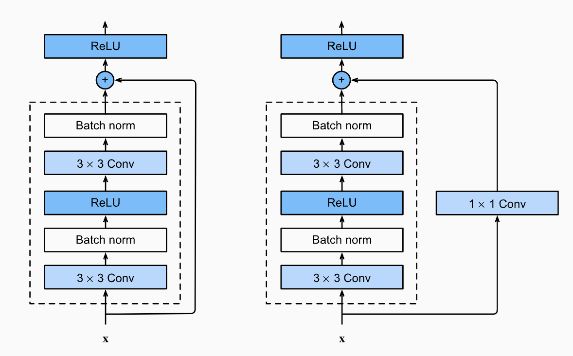
Fig. 52 Residual blocks may require “projections” such as 1 × 1 convs or linear layers to match shapes when combining.

Modifying our architecture to allow for skip connections (but still include the default model):

class ResidualConnection(nn.Module):
    def __init__(self, n: int, skip=False):
        super().__init__()
        self.linear = nn.Linear(n, n)
        self.ln = nn.LayerNorm(n)
        self.act_fn = F.relu
        self.skip = skip
    
    def forward(self, x):
        hx = self.linear(self.act_fn(self.ln(x)))
        return x + hx if self.skip else hx


def get_model(vocab_size: int,
              block_size: int,
              emb_size: int,
              width: int,
              num_linear: int,
              skip: bool = True):

    layers = [
        nn.Embedding(vocab_size, emb_size), 
        nn.Flatten(),
        nn.Linear(block_size * emb_size, width),
        ResidualConnection(width, skip)
    ]
    
    for _ in range(num_linear):
        layers.append(ResidualConnection(width, skip))

    layers.append(nn.LayerNorm(width))
    layers.append(nn.ReLU())
    layers.append(nn.Linear(width, vocab_size))
    layers.append(nn.LayerNorm(vocab_size))
    model = nn.Sequential(*layers)
    return model

Remark. This iteratively adds [LN, ReLU, Linear] blocks instead of [Linear, LN, ReLU] used above. These are clearly equivalent. More importantly, notice that the network is constant width, i.e. ResidualConnection only requires the width parameter. Having different input and output width requires an extra linear layer on the input x to match the weights. Our implementation follows the PreAct ResNet [HZRS16] setup shown in Fig. 53 (right). Placing the linear layer after the activation allows the residual to have negative values.

Fig. 53 The original ResNet block (left) applies a non-linear activation function, usually ReLU, after the skip connection. In contrast, the pre-activation ResNet block (right) applies the non-linearity at the beginning of \(H\). For very deep network, the pre-activation ResNet has shown to perform better as the gradient flow is guaranteed to have the identity matrix as calculated below, and is not harmed by any non-linear activation applied to it. Source: [HZRS16]

Despite its simplicity, the idea of a skip connection is highly effective as it supports stable gradient propagation through the network. Notice that there are now two paths across a layer: one through the non-linearity and one around it. In particular, the gradients across the skip connection passes undisturbed since:

\[ \frac{\partial \boldsymbol{\mathsf{x}}^{\ell+1}}{\partial \boldsymbol{\mathsf{x}}^\ell}=\mathbf{I}+\frac{\partial H(\boldsymbol{\mathsf{x}}^\ell)}{\partial \boldsymbol{\mathsf{x}}^\ell}. \]

Applying the residual formula recursively unravels a deep residual network into combinatorially many paths where the gradient can pass through the shortest (i.e. across all skip connections) or longest (i.e. across all nonlinearities) path through the network:

\[\begin{split} \begin{aligned} \boldsymbol{\mathsf{x}}^{\ell+2} &= \boldsymbol{\mathsf{x}}^{\ell + 1} + H^{\ell+1}(\boldsymbol{\mathsf{x}}^{\ell + 1}) \\ &= \boldsymbol{\mathsf{x}}^{\ell} + H^\ell(\boldsymbol{\mathsf{x}}^{\ell}) + H^{\ell+1}(\boldsymbol{\mathsf{x}}^{\ell} + H^\ell(\boldsymbol{\mathsf{x}}^{\ell})). \end{aligned} \end{split}\]

This is shown in Fig. 54. Allowing short paths for the gradient to flow to earlier layers of the network solves the problem of getting uninformative gradients with depth. In fact, Fig. 55 shows that a large percentage of gradient updates come from shorter paths. The paper [HZRS15a] demonstrated the benefits of this by succesfully training ResNet-152, a 152-layer deep residual CNN, getting SOTA performance on ImageNet in 2015.

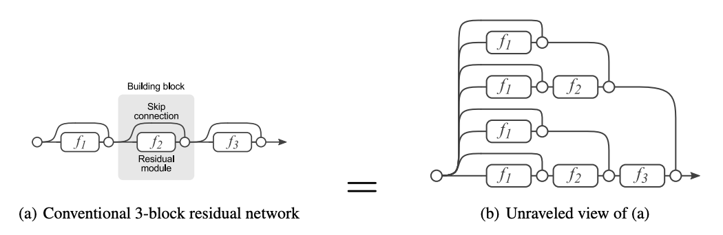
Fig. 54 Unraveled view of a residual network. Source: [VWB16]

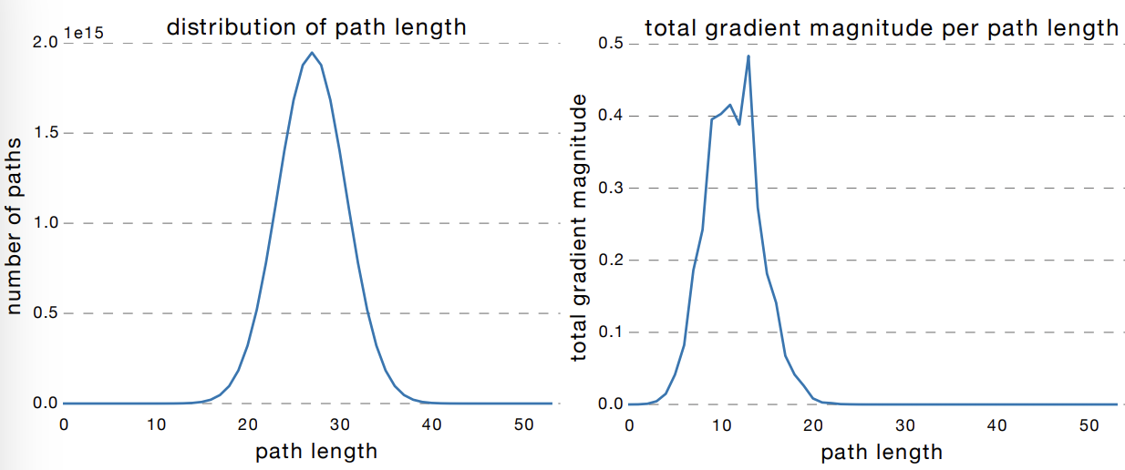
Fig. 55 Most of the gradient in a residual network with 54 layers comes from paths that are only 5-17 layers deep. Residual networks avoid the vanishing gradient problem by introducing short paths during training. Source: [VWB16]

Trying out whether residual connections diminish rank collapse and accelerate convergence:

import time

sv_hooks = {}
trainers = {}
message = ["\nloss (last 100 steps)"]
model_params["num_linear"] = 5
train_params["lr"] = 0.3
train_params["steps"] = 3000

for skip in [True, False]:
    
    start_time = time.time()
    sv_ratio = SingularValuesRatio()
    init_fn = lambda w: nn.init.xavier_uniform_(w, gain=np.sqrt(2), generator=g())
    model = init_model(get_model(skip=skip, **model_params), init_fn)
    hooks = [{"bwd_hooks": [], "fwd_hooks": [sv_ratio], "layer_types": (nn.Linear,)}]
    trainer = run(model, train_dataset, **train_params, hooks=hooks)
    
    trainers[skip] = trainer
    sv_hooks[skip] = sv_ratio
    train_time = time.time() - start_time
    message.append(f"    skip={'True: ' if skip else 'False:'}   {sum(trainer.logs['train']['loss'][-100:]) / 100:.3f}      (t={train_time:.3f}s)")

print("\n".join(message))

loss (last 100 steps)
    skip=True:    2.423      (t=90.175s)
    skip=False:   2.486      (t=86.408s)

Faster convergence. A shallow network initially has rapid decrease in loss followed by convergence to a shallow minimum. On the other hand, deep networks train slowly, but reaches a better minimum after many epochs. Residual connections speed up training by solving the slowness issue of deep networks at the beginning of training:

Show code cell source Hide code cell source

plt.figure(figsize=(5, 3))
for skip in [False, True]:
    trainer = trainers[skip]
    train_loss = trainer.logs["train"]["loss"]
    train_loss_ma = moving_avg(train_loss, window=0.05)
    plt.plot(train_loss_ma, label=f"MLP{' + skip' if skip else ''}")
    plt.ylabel("loss (MA)")
    plt.xlabel("steps")
    plt.grid(linestyle="dotted", alpha=0.6)
    plt.legend();

Rank collapse at initialization. From the functional form of the residual connection, assuming that the initial inputs are linearly independent, the layer should avoid rank collapse. As discussed above, this results in faster training since the gradients and inputs are more informative. The following plot confirms this:

Show code cell source Hide code cell source

fig, ax = plt.subplots(1, len(sv_hooks), figsize=(10, 4))
for i, skip in enumerate([False, True]):
    records = sv_hooks[skip].records
    for j, m in enumerate(records.keys()):
        ax[i].plot(moving_avg(records[m], window=0.0005), label=m.__class__.__name__ + "." + str(j), color=f"C{j}", alpha=min(0.5 + (0.5 / len(records.keys())) * j, 1.0))
        ax[i].set_ylim(0, 1)
        ax[i].grid(linestyle="dashed", alpha=0.5)
        ax[i].set_xlabel("steps")
        if skip:
            ax[i].set_title("LN + Residual MLP Block")
        else:
            ax[i].set_title("LN + MLP")

ax[0].set_ylabel(r"${\sigma}_1\; /\; {\sigma}$.sum()")
ax[-1].legend(fontsize=7)
fig.tight_layout()

Figure. Residual connections diminish rank collapse at initialization without using BN.

Residual connections + low rank as memory. The combination of residuality and low rank turns out as simulating large associative memory. The changes to the inputs are small relative to the large ambient dimension so that weight updates do not completely erase the current state of the network. Early layers can write information that can be used by later layers due to skip connections. Later layers can learn to edit this information, e.g. deleting it provided sufficient complexity, if doing so reduces the loss. But by default information is preserved. This also shows that a limitation or bottleneck such as low rank can be essential to learning provided the network architecture provides ways to exploit or sidestep it.

---

■