Regularization

How do we control bias and variance? There are two solutions: (1) getting more data, (2) tuning model complexity. More data decreases variance but has no effect on bias. Increasing complexity decreases bias but increases variance. Since biased models do not scale well with data, a good approach is to start with a complex model and decrease complexity it until we get a good tradeoff. This approach is called regularization. Regularization can be thought of as a continuous knob on complexity that smoothly restricts model class.

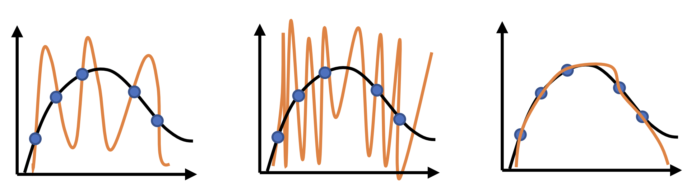
Fig. 11 All these have zero training error. But the third one is better. This is because resampling will result in higher empirical risk for the first two, which implies high true risk. Source: [CS182-lec3]

Bayesian perspective

High variance occurs when data does not give enough information to identify parameters. If we provide enough information to disambiguate between (almost) equally good models, we can pick the best one. One way to provide more information is to make certain parameter values more likely. In other words, we assign a prior on the parameters. Since the optimizer picks parameter values based on the loss, we can look into how we can augment the loss function to do this. Instead of MLE, we do a MAP estimate for \(\boldsymbol{\Theta}\):

\[\begin{split} \begin{aligned} p(\boldsymbol{\Theta} \mid \mathcal{D}) &\propto p(\boldsymbol{\Theta}) \; {p(\mathcal{D} \mid \boldsymbol{\Theta})} \\[4pt] &= p(\boldsymbol{\Theta}) \, \prod_i \frac{p(\boldsymbol{\mathsf{x}}_i, y_i, \boldsymbol{\Theta})}{ p(\boldsymbol{\Theta})\,p(\boldsymbol{\mathsf{x}}_i)} \,p(\boldsymbol{\mathsf{x}}_i) \\ &= p(\boldsymbol{\Theta}) \, \prod_i \frac{p(\boldsymbol{\mathsf{x}}_i, y_i, \boldsymbol{\Theta})}{ p(\boldsymbol{\mathsf{x}}_i, \boldsymbol{\Theta})} \,p(\boldsymbol{\mathsf{x}}_i) \\ &= p(\boldsymbol{\Theta}) \, \prod_i p_{\boldsymbol{\Theta}}(y_i \mid \boldsymbol{\mathsf{x}}_i) \,p(\boldsymbol{\mathsf{x}}_i). \\ \end{aligned} \end{split}\]

Note we used independence between params and input. This also means that the term for the input is an additive constant, and therefore ignored in the resulting loss:

\[ \mathcal{L}_{\mathcal{D}}(\boldsymbol{\Theta}) = - \left (\sum_i \log p_{\boldsymbol{\Theta}}(y_i \mid \boldsymbol{\mathsf{x}}_i) \right) - \underbrace{\log p(\boldsymbol{\Theta})}_{\text{we choose this}}. \]

Can we pick a prior that makes the smoother function more likely? This can be done by assuming a distribution on \(\boldsymbol{\Theta}\) that assigns higher probabilities to small weights: e.g. \(p(\boldsymbol{\Theta}) \sim \mathcal{N}(\mathbf{0}, \sigma^2\mathbf{I}).\) This may result in a smoother fit (Fig. 11c). Solving the prior:

\[\begin{split} \begin{aligned} \log p(\boldsymbol{\Theta}) &= \sum_{j} \left(-\frac{1}{2\sigma^2} {\theta_j}^2 - \log \sigma - \frac{1}{2} \log 2 \pi \right) \\ &= - \lambda \lVert \boldsymbol{\Theta} \rVert^2 + \text{const.} \\ \end{aligned} \end{split}\]

where \(\lambda > 0\) and \(\lVert \cdot \rVert\) is the L2 norm. Since we choose the prior, \(\lambda\) effectively becomes a hyperparameter that controls the strength of regularization. The resulting loss has the L2 regularization term:

\[ \mathcal{L}_{\mathcal{D}}(\boldsymbol{\Theta}) = - \left( \sum_i \log p_{\boldsymbol{\Theta}}(y_i \mid \boldsymbol{\mathsf{x}}_i) \right) - \lambda \lVert \boldsymbol{\Theta} \rVert^2. \]

The same analysis with a Laplace prior results in the L1 regularization term:

\[- \lambda \lVert \boldsymbol{\Theta} \rVert_1 = -\lambda \sum_j |\theta_j|.\]

Remark. It makes sense that MAP estimates result in weight penalty since the weight distribution is biased towards low values. Intuitively, large weights means that the network is memorizing the training dataset, and we get sharper probability distributions with respect to varying input features. Since the class of models are restricted to having low weights, this puts a constraint on the model class, resulting in decreased complexity. Note that these regularizers introduce hyperparameters that we have to tune well. See experiments below.

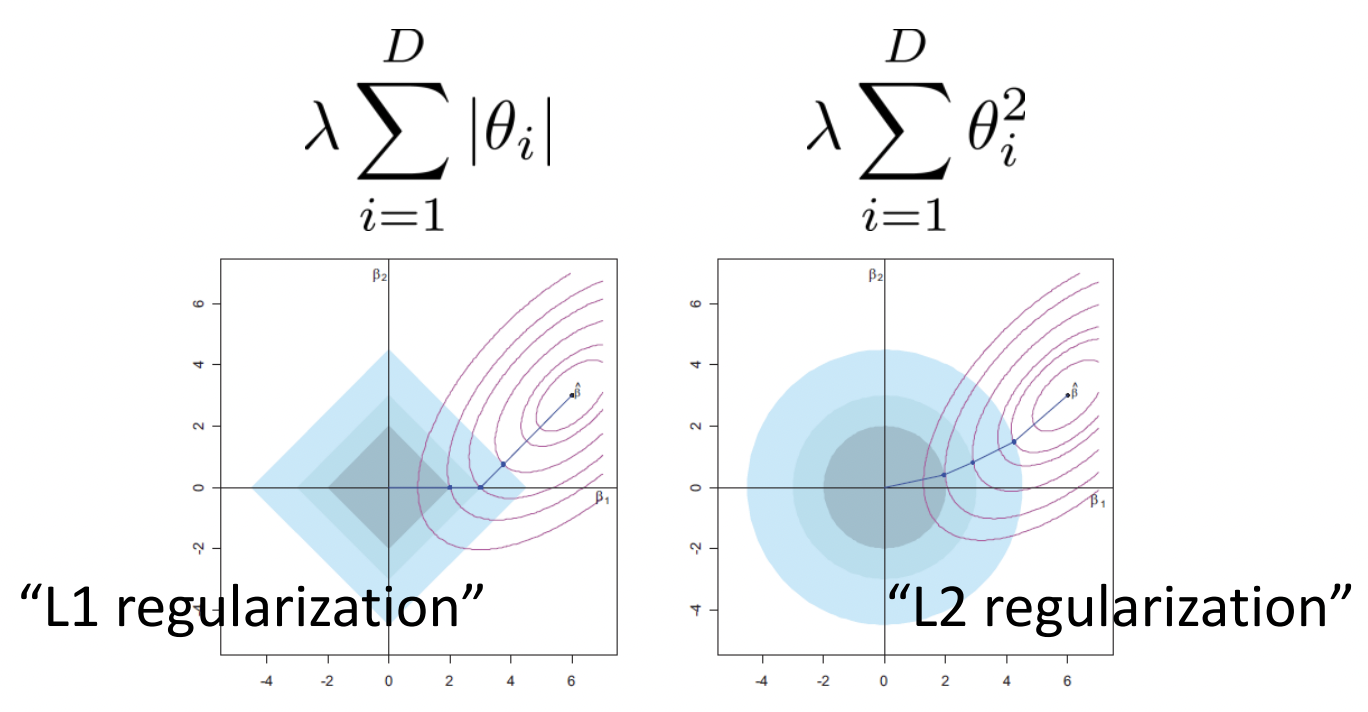
Fig. 12 Minimizing both prediction loss and regularization loss surfaces. The green point shows the optimal weights for fixed prediction loss. L1 results in sparse weights, while L2 distributes the contraint among both weights. Source

Other perspectives

A numerical perspective is that adding a regularization term can make underdetermined problems well-determined (i.e. has a better defined minimum). The optimization perspective is that the regularizer makes the loss landscape easier to search. Paradoxically, regularizers can sometimes reduce underfitting if it was due to poor optimization! Other types of regularizers are ensembling (e.g. Dropout) and gradient penalty (for GANs).

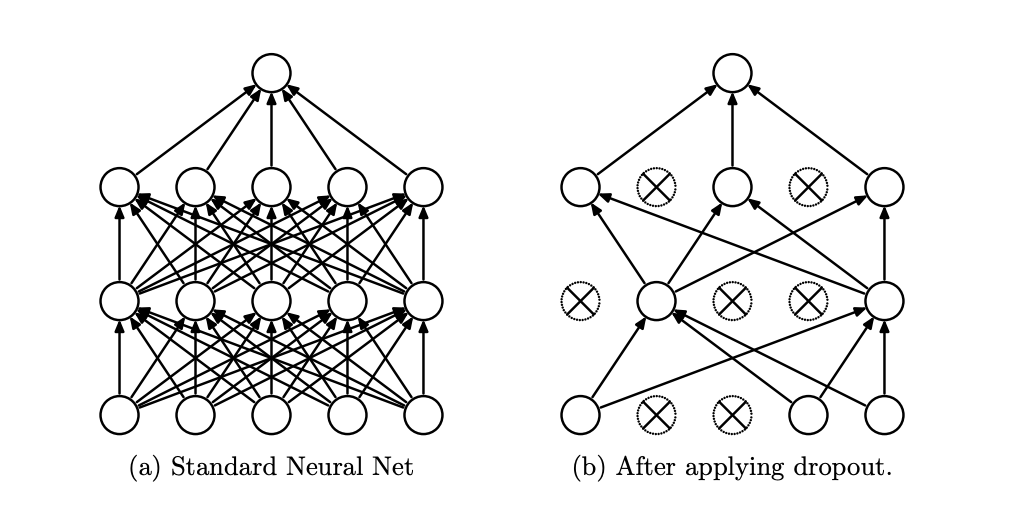
Fig. 13 [SHK+14] Dropout drops random units with probability \(p\) at each step during training. This prevents overfitting by reducing the co-adaptation of neurons during training, which in turn limits the capacity of the model to fit noise in the training data. Since only \(1 - p\) units are present during training, the activations are scaled by \(\frac{1}{1 - p}\) to match test behavior.