Bias-variance decomposition

Recall that the training set $\mathcal{D}$ is sampled from an underlying distribution $P$ (i.e. the data generating process). Thus, we want to know how model performance of the trained model $f_{\mathcal{D}}$ varies with respect to training sample $\mathcal{D}.$ Here, we will analyze the squared error of regression models. For simplicity, we assume the existence of a a ground truth function $f$ that assigns the label of an input $\mathsf{x}$ (see remark below).

Let $f_{\mathcal{D}}$ be the function obtained by the training process over the sample $\mathcal{D}.$ Let $\overline{f}$ be the expected function when drawing fixed sized samples $\mathcal{D}\stackrel{\text{iid}}{\sim }{P}^N$ where $N=|\mathcal{D}|$ and $P$ is the underlying data distribution. In other words, $\overline{f}$ is an ensemble of trained models weighted by the probability of its training dataset. Then:

$$\begin{array}{r}\begin{array}{rl}{\mathbb{E}}_{\mathsf{x},\mathcal{D}}\left[{(f_{\mathcal{D}}(\mathsf{x})-f(\mathsf{x}))}^2\right]& ={\mathbb{E}}_{\mathsf{x},\mathcal{D}}\left[{((f_{\mathcal{D}}(\mathsf{x})-\overline{f}(\mathsf{x}))+(\overline{f}(\mathsf{x})-f(\mathsf{x})))}^2\right]\\ & ={\mathbb{E}}_{\mathsf{x},\mathcal{D}}[(f_{\mathcal{D}}(\mathsf{x})-\overline{f}(\mathsf{x}){)}^2]+{\mathbb{E}}_{\mathsf{x},\mathcal{D}}[(\overline{f}(\mathsf{x})-f(\mathsf{x}){)}^2]\\ & +2\cdot {\mathbb{E}}_{\mathsf{x},\mathcal{D}}[(f_{\mathcal{D}}(\mathsf{x})-\overline{f}(\mathsf{x}))(\overline{f}(\mathsf{x})-f(\mathsf{x}))]\\ \\ & ={\mathbb{E}}_{\mathsf{x},\mathcal{D}}[(f_{\mathcal{D}}(\mathsf{x})-\overline{f}(\mathsf{x}){)}^2]+{\mathbb{E}}_{\mathsf{x},\mathcal{D}}[(\overline{f}(\mathsf{x})-f(\mathsf{x}){)}^2]+0\\ & =\underset{\text{Variance}}{\underbrace{{\mathbb{E}}_{\mathsf{x},\mathcal{D}}[(f_{\mathcal{D}}(\mathsf{x})-\overline{f}(\mathsf{x}){)}^2]}}+\underset{{\text{Bias}}^2}{\underbrace{{\mathbb{E}}_{\mathsf{x}}[(\overline{f}(\mathsf{x})-f(\mathsf{x}){)}^2]}}.\end{array}\end{array}$$

The middle term vanishes by writing it as:

$${\mathbb{E}}_{\mathsf{x}}[\underset{0}{\underbrace{{\mathbb{E}}_{\mathcal{D}}[(f_{\mathcal{D}}(\mathsf{x})-\overline{f}(\mathsf{x}))]}}(\overline{f}(\mathsf{x})-f(\mathsf{x}))]=0.$$

Observe that the variance term describes variability of models as we re-run the training process without actually looking into the true function. The bias term, on the other hand, looks at the error of the ensemble $\overline{f}$ from the true function $f.$ These can be visualized as manifesting in the left and right plots respectively of Fig. 7.

Remark. This derivation ignores target noise which is relevant in real-world datasets. Here we have a distribution $p(y\mid \mathsf{x})$ around the target on which we integrate over to get the expected target. See these notes for a more careful treatment.

Classical tradeoff

The classical tradeoff is that, as model complexity increases, models fit each sample so closely that they capture even sampling noise. However, these errors tend to cancel out over many samples, resulting in low bias. Overfitting occurs when the model performs well on the training data but may not generalize to a test sample due to high variance. Conversely, simpler models tend to have high bias and underfit any sample from the dataset.

For a fixed model class, assuming the data is well-structured, increasing the sample size generally decreases variance, as more data smooths out noise. Interestingly, bias stems from the choice of model class (e.g., architecture, choice of hyperparameters) and persists regardless of the amount of data available. Indeed, [Bar91] provides an explicit tradeoff between data and network size (i.e. its width) for sigmoidal FCNNs with two layers:

$${\mathbb{E}}_{\mathsf{x},\mathcal{D}}\left[{(f_{\mathcal{D}}(\mathsf{x})-f(\mathsf{x}))}^2\right]\le O\left(\frac{1}{M}\right)+O\left(\frac{Md}{N}\right)\log N$$

where $M$ is the number of nodes, $N=|\mathcal{D}|$ is the number of training observations, and $d$ is the input dimension. Here the first term corresponds to the bias which is data independent, while the second term corresponds to the variance which increases with network size and decreases with data. The above bound also highlights the curse of dimensionality. The input dimension contributes linearly to the error, while data only decreases error at the rate $O(\log N/N)$.

Double descent

For large models there is the phenomenon of double descent [NKB+19] observed in most networks used in practice where both bias and variance go down with excess complexity. One intuition is that near the interpolation threshold, where there is roughly a 1-1 correspondence between the sample datasets and the models, small changes in the dataset lead to large changes in the model. The strip around this is the critical regime in the classical case where overfitting occurs. Having more data destroys this 1-1 correspondence, which is covered by the classical tradeoff discussed above.

Double descent occurs in the opposite case where we have much more parameters than data (Fig. 8). SGD gets to focus more on what it wants to do, i.e. search for flat minima [KMN+16a], since it is not constrained to use the full model capacity. Interestingly, the double descent curve is more prominent when there is label noise. In this case, there is less redundancy in the model parameters when the dataset is harder to learn, so that the complexity tradeoff is sharper in the critical strip.

Remark. Models around with weights flat minimas have validation errors that are much more stable to perturbation in the weights and, as such, tend to be smooth between data points [HS97a]. SGD is discussed in the next chapter.

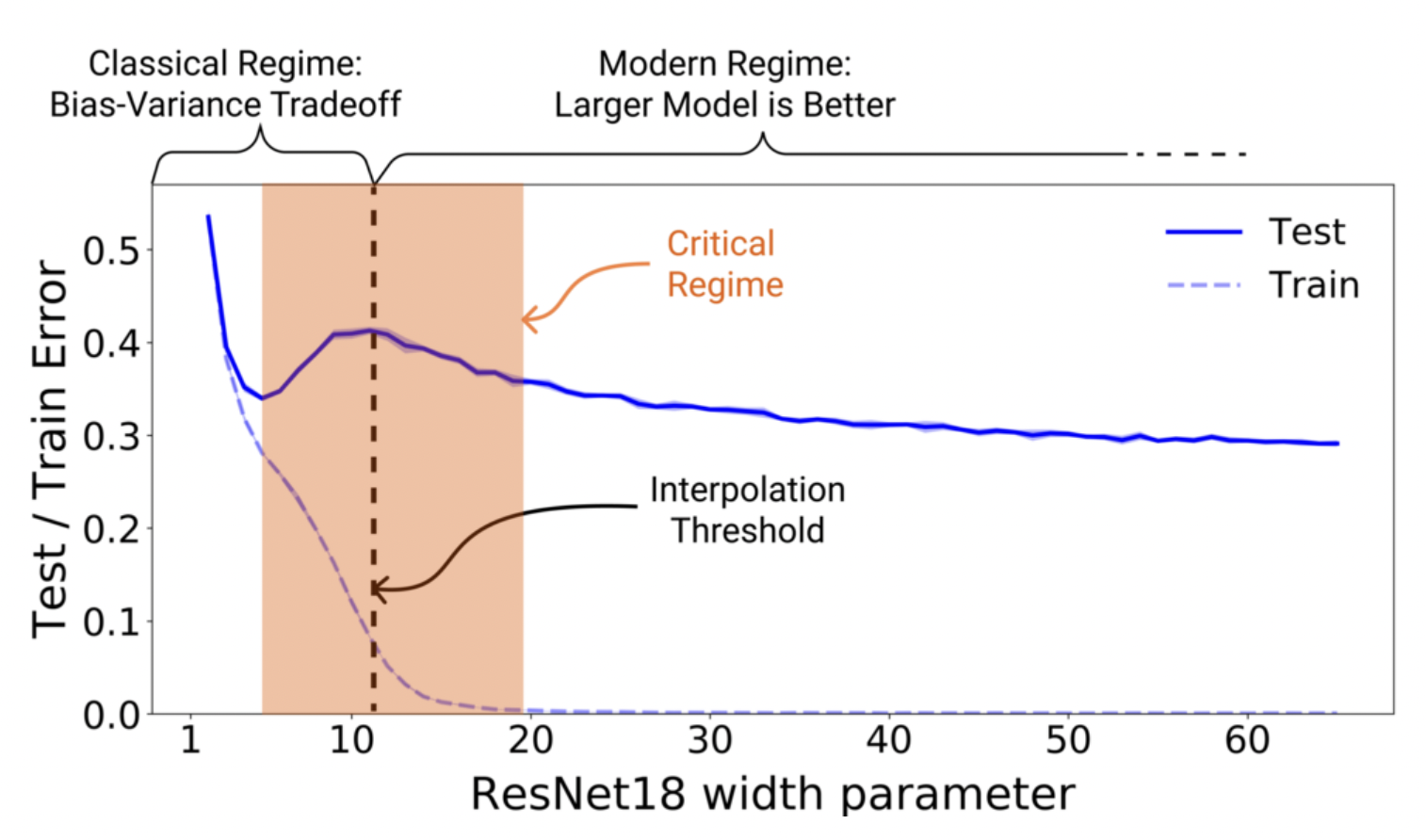
Fig. 8 Double descent for ResNet18. The width parameter controls model complexity. Source: [NKB+19]

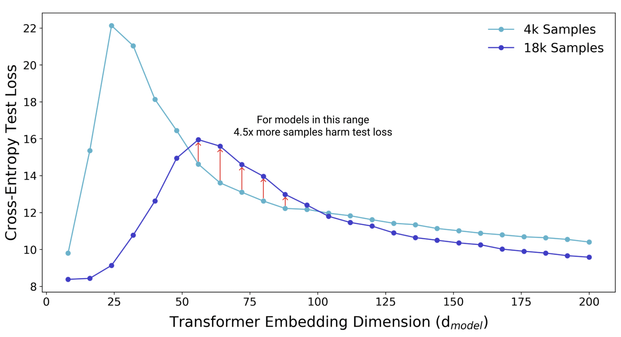
Fig. 9 Additional data increases model variance within the critical regime. More data shifts the interpolation threshold to the right, resulting in worse test performance compared to the same model trained on a smaller sample. Increasing model complexity improves test performance. Source: [NKB+19]

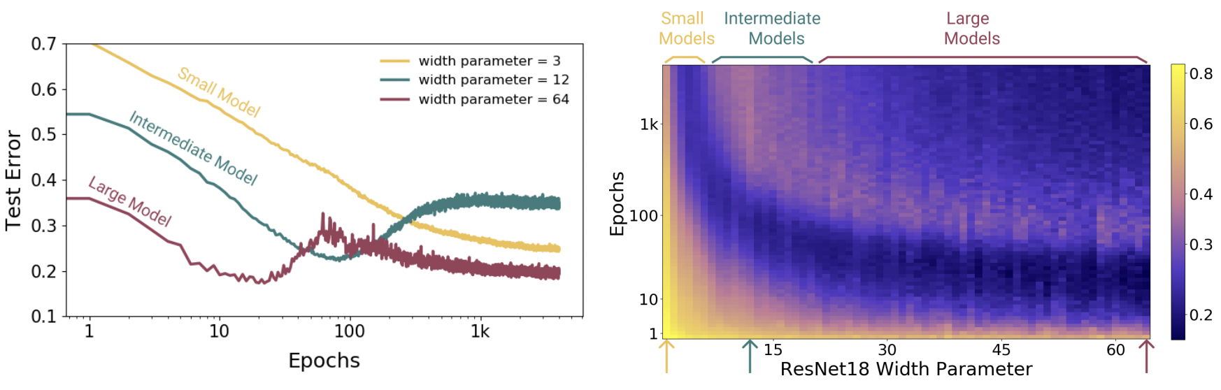
Fig. 10 Epoch dimension to double descent. Models are ResNet18s on CIFAR10 with 20% label noise, trained using Adam with learning rate 0.0001, and data augmentation. Left: Training dynamics for models in three regimes. Right: Test error vs. Model size × Epochs. Three slices of this plot are shown on the left. Source: [NKB+19]