Machine learning theory
For each choice of parameters \(\boldsymbol{\Theta}\), we defined the empirical risk \(\mathcal{L}_\mathcal{D}(\boldsymbol{\Theta})\) as an unbiased estimate of the true risk \(\mathcal{L}(\boldsymbol{\Theta})\) defined as the expected loss on the underlying distribution given the model \(f_{\boldsymbol{\Theta}}\). It is natural to ask whether this is an accurate estimate. There are two things to watch out for when training our models:
Overfitting. This is characterized by having low empirical risk, but high true risk. This can happen if the dataset is too small to be representative of the true distribution. Or if the model is too complex. In the latter case, the model will interpolate the sample, but will have arbitrary behavior between datapoints.
Underfitting. Here the empirical risk, and thereby the true risk, is high. This can happen if the model is too weak (low capacity, or too few parameters) — e.g. too strong regularization. Or if the optimizer is not configured well (e.g. wrong learning rate), so that the parameters \(\boldsymbol{\Theta}\) found are inadequate even on the training set.
Observe that MLE is by definition prone to overfitting. We rely on smoothness between data points for the model to generalize to test data. It is important to analyze the error between different training samples. A well-trained model should not look too different between samples. But we also don’t want it to have the same errors with different data! (Fig. 7)
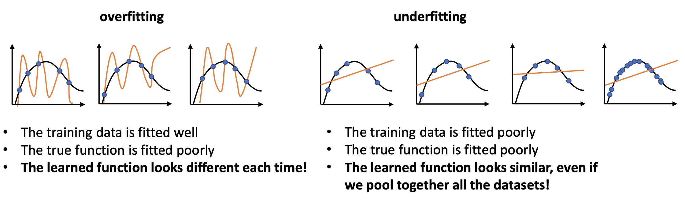
Fig. 7 Drawing of a model that overfits and underfits the distribution. Source
Model complexity
Here model capacity or complexity is a measure of how complicated a pattern or relationship a model architecture can express. Let \(f\) be the true function that underlies the task. If model capacity is sufficiently large, the model class \(\mathscr{F} = \{f_{\boldsymbol{\Theta}} \mid \boldsymbol{\Theta} \in \mathbb{R}^d \}\) contains an approximation \(\hat{f} \in \mathscr{F}\) such that \(\| f - \hat{f} \| < \epsilon\) for a small enough \(\epsilon > 0.\)
Here model architecture refers to the computation graph with unspecified parameters \(\boldsymbol{\Theta}\). That is, the map \(\boldsymbol{\Theta} \mapsto f_{\boldsymbol{\Theta}}\) results to an actual function once the parameters are specified, e.g. a trained model if \(\boldsymbol{\Theta}^*\) is optimally chosen. All these distinct objects are typically referred to simply as a ‘model’, with the distinction being determined by context.
Model capacity[1] can be controlled by the number of parameters in practical architectures. It can also be constrained directly by applying regularization or certain inductive biases. Inductive bias refers to built-in knowledge or biases in a model designed to help it learn. All such knowledge is bias in the sense that it makes some solutions more likely, and others less likely.