Backpropagation

In this notebook, we look at the backpropagation algorithm (BP) for efficient gradient computation on computational graphs. Backpropagation involves local message passing of values in the forward pass, and gradients in the backward pass. Neural networks are computational graphs with nodes for differentiable operations. The time complexity of BP is linear in the size of the network, i.e. the total number of edges and compute nodes. This fact allows scaling training large neural networks. We will implement a minimal scalar-valued autograd engine and a neural network library[1] on top it to train a small regression model.

BP on computational graphs

A neural network can be implemented as a directed acyclic graph (DAG) of nodes that models a function \(f\), i.e. all computation flows from an input \(\boldsymbol{\mathsf{x}}\) to an output node \(f(\boldsymbol{\mathsf{x}})\) with no cycles. During training, this is extended to implement the calculation of the loss. Recall that our goal is to obtain optimal parameter node values \(\hat{\boldsymbol{\Theta}}\) after optimization (e.g. with SGD) such that the \(f_{\hat{\boldsymbol{\Theta}}}\) minimizes the expected value of the loss function \(\ell.\) Backpropagation allows us to efficiently compute \(\nabla_{\boldsymbol{\Theta}} \ell\) for SGD after \((\boldsymbol{\mathsf{x}}, y) \in \mathcal{B}\) is passed to the input nodes.

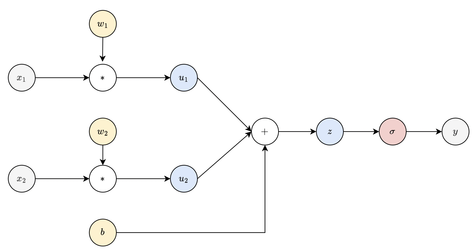
Fig. 32 Computational graph of a dense layer. Note that parameter nodes (yellow) always have zero fan-in.

Forward pass. Forward pass computes \(f_{\boldsymbol{\Theta}}(\boldsymbol{\mathsf{x}}).\) All compute nodes are executed starting from the input nodes (which evaluates to the input vector \(\boldsymbol{\mathsf x}\)). This passed to its child nodes, and so on up to the loss node. The output value of each node is stored to avoid recomputation for child nodes that depend on the same node. This also preserves the network state for backward pass. Finally, forward pass builds the computational graph which is stored in memory. It follows that forward pass for one input is roughly \(O(\mathsf{E})\) in time and memory where \(\mathsf{E}\) is the number of edges of the graph.

Backward pass. Backward computes gradients starting from the loss node \(\ell\) down to the input nodes \(\boldsymbol{\mathsf{x}}.\) The gradient of \(\ell\) with respect to itself is \(1\). This serves as the base step. For any other node \(u\) in the graph, we can assume that the global gradient \({\partial \ell}/{\partial v}\) is cached for each node \(v \in N_u\), where \(N_u\) are all nodes in the graph that depend on \(u\). On the other hand, the local gradient \({\partial v}/{\partial u}\) is determined analytically based on the functional dependence of \(v\) upon \(u.\) These are computed at runtime given current node values cached during forward pass.

The global gradient with respect to node \(u\) can then be inductively calculated using the chain rule:

\[ \frac{\partial \ell}{\partial u} = \sum_{v \in N_u} \frac{\partial \ell}{\partial v} \frac{\partial v}{\partial u}. \]

This can be visualized as gradients flowing from the loss node to each network node. The flow of gradients will end on parameter and input nodes which depend on no other nodes. These are called leaf nodes. It follows that the algorithm terminates.

Fig. 33 Computing the global gradient for a single node. Note that gradient type is distinguished by color: local (red) and global (blue).

This can be visualized as gradients flowing to each network node from the loss node. The flow of gradients will end on parameter and input nodes which have zero fan-in. Global gradients are stored in each compute node in the grad attribute for use by the next layer, along with node values obtained during forward pass which are used in local gradient computation. Memory can be released after the weights are updated. On the other hand, there is no need to store local gradients as these are computed as needed.

Backward pass is implemented as follows:

class Node:
    ...

    def sorted_nodes(self):
        """Return topologically sorted nodes with self as root."""
        ...

    def backward(self):
        self.grad = 1.0
        for node in self.sorted_nodes():
            for parent in node._parents:
                parent.grad += node.grad * node._local_grad(parent)

Each node has to wait for all incoming gradients from dependent nodes before passing the gradient to its parents. This is done by topological sorting of the nodes, based on functional dependency, with self as root (i.e. the node calling backward is always treated as the terminal node). The contributions of child nodes are then accumulated based on the chain rule, where node.grad is the global gradient which is equal to ∂self / ∂node, while the local gradient node._local_grad(parent) is equal to ∂node / ∂parent. By construction, each child node occurs before any of its parent nodes, thus the full gradient of a child node is calculated before it is sent to its parent nodes (Fig. 34).

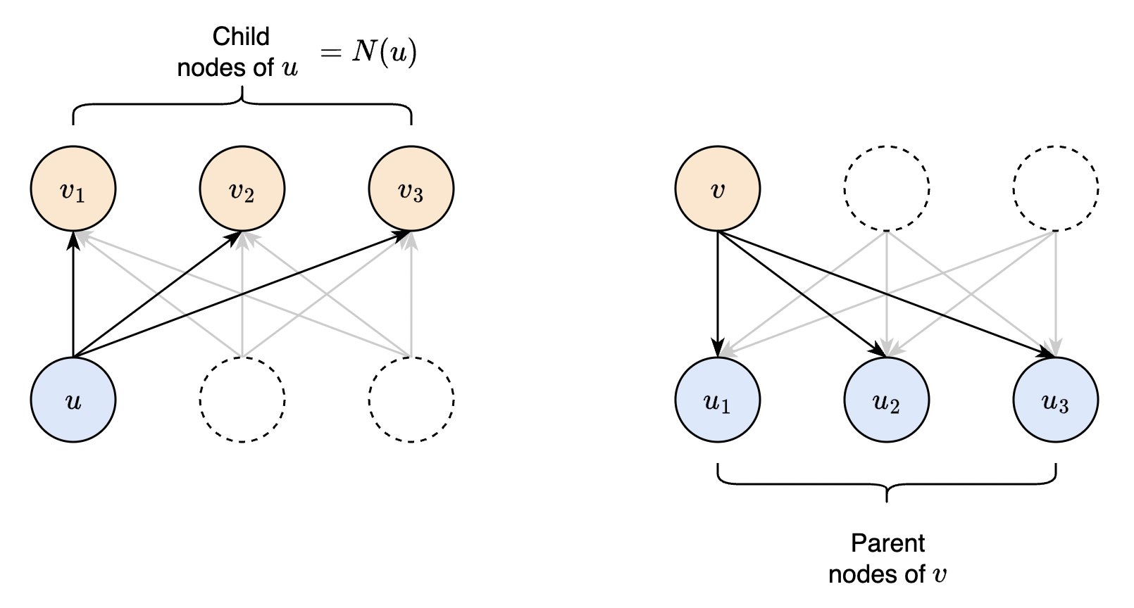
Fig. 34 Equivalent ways of computing the global gradient. (left) The global gradient is computed by tracking the dependencies from \(u\) to each of its child node during forward pass. This is our formal statement before. Algorithmically, we start from each node in the upper layer, and we contribute one term in the sum to each parent node (right). Note that this assumes that the global gradient at \(v\) has been fully accumulated / calculated.

Topological sorting with DFS

To construct the topologically sorted list of nodes of a DAG starting from a terminal node, we use depth-first search. The following example is shown in Fig. 35. The following algorithm steps into dfs for each parent node until a leaf node is reached, which is pushed immediately to topo. Then, the algorithm steps out and the next parent node is processed. A node is only pushed when all its parents have been pushed (i.e. already in topo or finished looping through its parents), preserving the required linear ordering.

from collections import OrderedDict

parents = {
    "a": [],
    "b": [],
    "x": [],
    "c": ["a", "b"],
    "d": ["x", "a", "c"],
    "e": ["c"],
    "f": ["d"]
}

def sorted_nodes(root):
    """Return topologically sorted nodes with self as root."""
    topo = OrderedDict()
    
    def dfs(node):
        print("v", node)
        if node not in topo:
            for parent in parents[node]:
                dfs(parent)
            
            topo[node] = None
            print("t", list(topo.keys()))

    dfs(root)
    return reversed(topo)

list(sorted_nodes("f"))

v f
v d
v x
t ['x']
v a
t ['x', 'a']
v c
v a
v b
t ['x', 'a', 'b']
t ['x', 'a', 'b', 'c']
t ['x', 'a', 'b', 'c', 'd']
t ['x', 'a', 'b', 'c', 'd', 'f']

['f', 'd', 'c', 'b', 'a', 'x']

Remark. Note that we get infinite recursion if there is a cycle in the graph, so the acyclic hypothesis is important for the algorithm to terminate. A way to detect cycles is to maintain a set of visited nodes. Revisiting a node that is not pushed to the output queue means that the graph is cyclic (see above outputs where v indicates visiting the node).

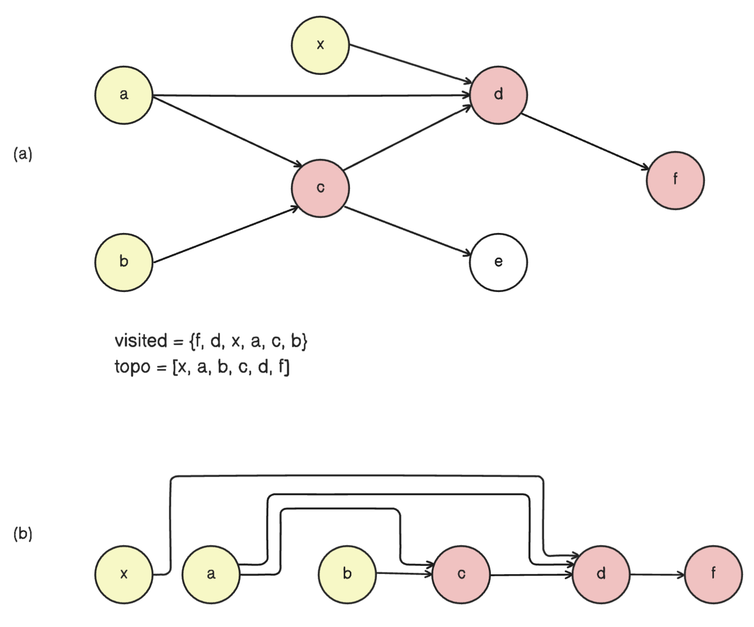
Fig. 35 (a) Graph encoded in the parents dictionary above. Note e, which f has no dependence on, is excluded. Visited nodes (red) starts from the terminal node backwards into the graph. Then, each node is pushed once all its parents are pushed (starting from leaf nodes, yellow), preserving topological ordering. Here a is not pushed twice, even if both d and c depends on it, since a has already been visited after node d. (b) Topological sorting exposes a linear ordering of the compute nodes.

Properties of backpropagation

Some characteristics of backprop which explains why it is ubiquitous in deep learning:

• Modularity. Backprop is a useful tool for reasoning about gradient flow and can suggest ways to improve training or network design. Moreover, since it only requires local gradients between nodes, it allows modularity when designing deep neural networks. In other words, we can (in principle) arbitrarily connect layers of computation. Another interesting fact is that a set of operations can be fused into a single node, resulting in more efficient computation (assuming there is an efficient way to solve for the local gradient in one step).

• Runtime. Each edge in the DAG is passed exactly once (Fig. 34). Hence, the time complexity for finding global gradients is \(O(\mathsf{E} + \mathsf{V})\) where \(\mathsf{E}\) is the number of edges in the graph and \(\mathsf{V}\) is the number of vertices. Moreover, we assume that each compute node and local gradient evaluation is \(O(1)\). It follows that computing \(\nabla_{\boldsymbol{\Theta}}\,\mathcal{L}\) for an instance \((\boldsymbol{\mathsf{x}}, y)\) is proportional to the network size, i.e. the same complexity as computing \(f(\boldsymbol{\mathsf{x}})\). Note that topological sorting of the nodes require the same time complexity.

• Memory. Each training step naively requires twice the memory for an inference step, since we store both gradients and values. This can be improved by releasing the gradients and neurons of non-leaf nodes in the previous layer once a layer finishes computing its gradient.

• GPU parallelism. Forward computation can generally be parallelized in the batch dimension and often times in the layer dimension. This can leverage massive parallelism in the GPU significantly decreasing runtime by trading off memory. The same is true for backward pass which can also be expressed in terms of matrix multiplications! (2)

Readings

• Back-propagation, an introduction

• Evaluating \(\nabla f(x)\) is as fast as \(f(x).\)

• Pytorch autograd explained - in-depth tutorial

• The spelled-out intro to neural networks and backpropagation: building micrograd

---

[1]

Inspired by https://github.com/karpathy/micrograd.