Fully-connected NNs (MLPs)

Fully-connected networks consist of a sequence of dense layers followed by an activation function. A dense layer consist of neurons which compute \(\mathsf{y}_k = \varphi(\boldsymbol{\mathsf{x}} \cdot \boldsymbol{\mathsf{w}}_k + b_k)\) for \(k = 1, \ldots, H\) where the activation \(\varphi\colon \mathbb{R} \to \mathbb{R}\) is a nonlinear function. The number of neurons \(H\) is called the width of the layer. The number of layers in a network is called its depth. Fully-connected networks are also historically known as multilayer perceptrons (MLPs).

This can be written in terms of matrix multiplication: \(\boldsymbol{\mathsf{X}}^1 = \varphi\left(\boldsymbol{\mathsf{X}}^0\,\boldsymbol{\mathsf{W}} + \boldsymbol{\mathsf{b}}\right)\) where \(B\) data points in \(\mathbb{R}^d\) are stacked so that the input \(\boldsymbol{\mathsf{X}}^0\) has shape \((B, d)\) allowing the network to process data in parallel. The layer output is then passed as input to the next layer.

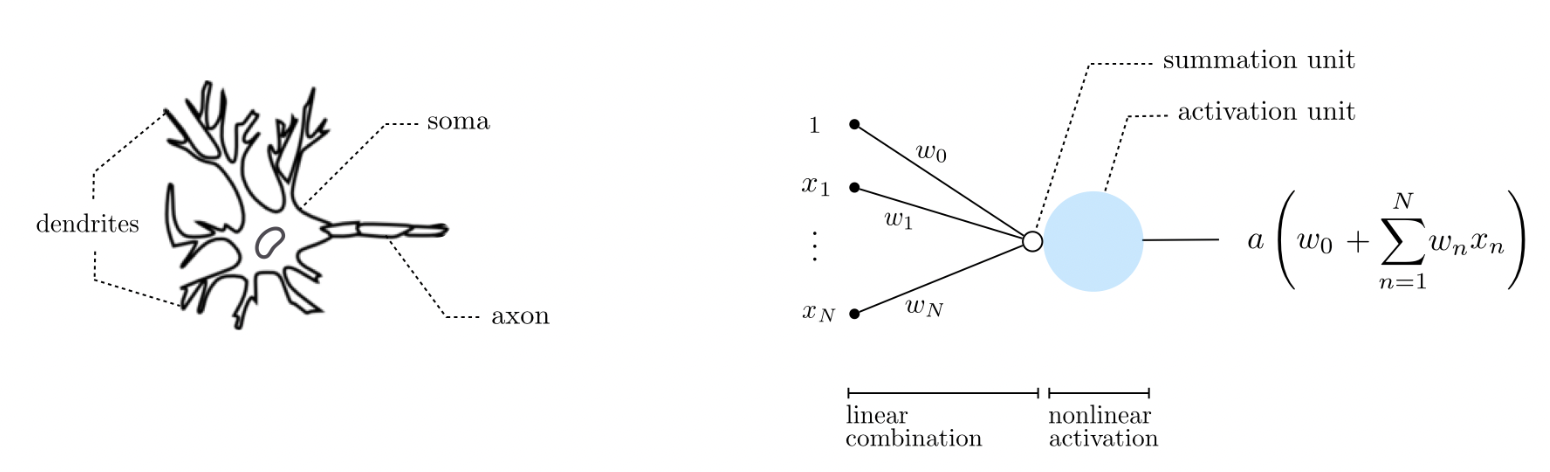
Fig. 5 An artificial neuron is a simplistic mathematical model for the biological neuron. Biological neurons are believed to remain inactive until the net input to the cell body (soma) reaches a certain threshold, at which point the neuron gets activated and fires an electro-chemical signal. Source

It turns out that fully-connected neural networks can approximate any continuous function \(f\) from a closed and bounded set \(K \subset \mathbb{R}^d\) to \(\mathbb{R}^m.\) This is a reasonable assumption about a ground truth function which we assume to exist. The following approximates a one-dimensional curve using a neural network with ReLU activation: \(z \mapsto \max(0, z)\) for \(z \in \mathbb{R}.\)

import torch

# Ground truth
x = torch.linspace(-2*torch.pi, 2*torch.pi, 1000)
y = torch.sin(x) + 0.3 * x

# Get (sorted) sample
B = torch.randint(0, 1000, size=(24,))
B = torch.sort(B)[0]
xs = x[B]
ys = y[B]

# ReLU approximation
z = torch.zeros(1000,) + ys[0]
for i in range(len(xs) - 1):
    if torch.isclose(xs[i + 1], xs[i]):
        m = torch.tensor(0.0)
    else:
        M = (ys[i+1] - ys[i]) / (xs[i+1] - xs[i])
        s, m = torch.sign(M), torch.abs(M)
    z += s * (torch.relu(m * (x - xs[i])) - torch.relu(m * (x - xs[i+1])))

Note that this only works for target function with compact domain [a, b].

Show code cell source Hide code cell source

import numpy as np
import matplotlib.pyplot as plt
from matplotlib_inline import backend_inline
backend_inline.set_matplotlib_formats('svg')

# Plotting
fig, ax = plt.subplots(1, 2, figsize=(10, 4))
ax[0].scatter(xs, ys, facecolor='none', s=12, edgecolor='k', zorder=3, label='data')
ax[0].plot(x, y, color="C1", label='f')
ax[0].set_xlabel('x')
ax[0].set_ylabel('y')
ax[0].legend();

ax[1].scatter(xs, ys, facecolor='none', s=12, edgecolor='k', zorder=4, label='data')
ax[1].plot(x, z, color="C0", label=f'relu approx. (B={len(B)})', zorder=3)
ax[1].plot(x, y, color="C1")
ax[1].set_xlabel('x')
ax[1].set_ylabel('y')
ax[1].legend();

This works by constructing step-like functions ___/‾‾‾ and ‾‾‾\___  but with slope in between adjacent points. The functions increment each other starting with the constant function ys[0]. Note this correctly ends with a constant function ys[-1].

Remark. This is an example of universal approximation by increasing layer width.