Gradient Optimization
Recall that we can visualize \(\mathcal{L}_{\mathcal{D}}(\boldsymbol{\Theta})\) as a surface (Fig. 20). Gradient descent (GD) finds the minimum by locally moving in the direction of greatest decrease in loss (Fig. 21). The step size in GD depends on the learning rate that has to be tuned well: a too large learning rate can result in overshooting the minimum and causing oscillations, while a too small learning rate can lead to slow convergence or getting stuck in local minima or plateaus. In this chapter, we will discuss gradient descent with momentum, as well as adaptive momentum with Adam [KB15] and RMSProp [Hin12], which adjust the learning rate during training and dampen oscillations to improve optimization performance.
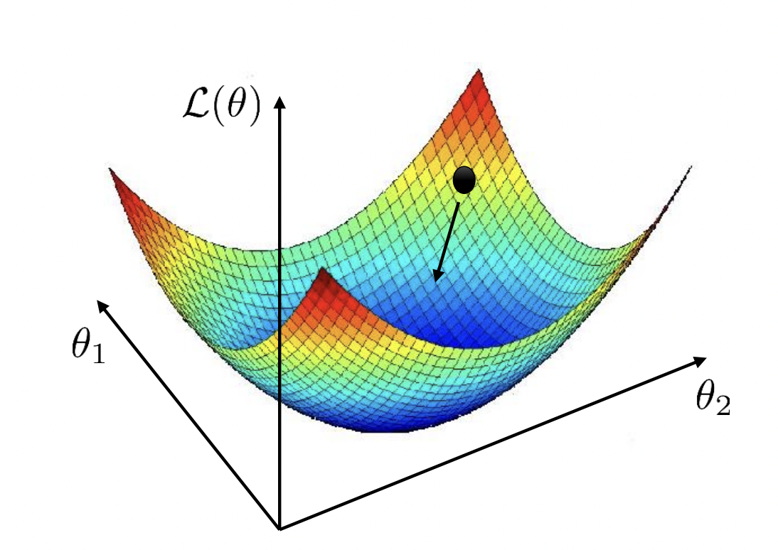
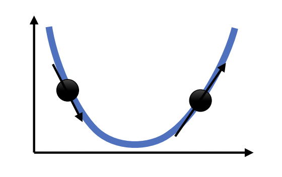
Fig. 21 Gradient descent in 1-dimension. Next step moves opposite to the direction of the slope. Moreover, step size is scaled based on the magnitude of the slope. Source
Optimizer template class
To experiment with GD algorithms, we create a template class. The template implements a method for zeroing out the gradients.
The only method that typically needs to be changed is update_param which contains the algorithm for updating parameters.
import torch
import torch.nn as nn

class OptimizerBase:
    def __init__(self, params: list, lr: float):
        self.params = params
        self.lr = lr

    def zero_grad(self):
        for p in self.params:
            if p.grad is None:
                continue
            p.grad.detach_()
            p.grad.zero_()

    @torch.no_grad()
    def step(self):
        for p in self.params:
            if p.grad is None:
                continue
            self.update_param(p)

    def update_param(self, p):
        raise NotImplementedError
Gradient descent can be implemented with the template as follows:
class GD(OptimizerBase):
    def __init__(self, params, lr):
        super().__init__(params, lr)

    def update_param(self, p):
        p += -self.lr * p.grad
We will test with the following synthetic loss surface (i.e. not generated with data):
# https://uvadlc-notebooks.readthedocs.io/en/latest/tutorial_notebooks/tutorial4/Optimization_and_Initialization.html
def pathological_loss(w0, w1):
    l1 = torch.tanh(w0) ** 2 + 0.01 * torch.abs(w1)
    l2 = torch.sigmoid(w1)
    return l1 + l2
Show code cell outputs
import numpy as np
import matplotlib.pyplot as plt
from matplotlib_inline import backend_inline
from mpl_toolkits.mplot3d import Axes3D
backend_inline.set_matplotlib_formats('svg')


def plot_surface(ax, f, title="", x_min=-5, x_max=5, y_min=-5, y_max=5, N=50):
    x = np.linspace(x_min, x_max, N)
    y = np.linspace(y_min, y_max, N)
    X, Y = np.meshgrid(x, y)
    Z = np.zeros_like(X)
    for i in range(N):
        for j in range(N):
            Z[i, j] = f(torch.tensor(X[i, j]), torch.tensor(Y[i, j]))

    ax.plot_surface(X, Y, Z, cmap='viridis')
    ax.set_xlabel(f'$w_0$')
    ax.set_ylabel(f'$w_1$')
    ax.set_title(title)


def plot_contourf(ax, f, w_hist, color, title="", levels=20, x_min=-5, x_max=5, y_min=-5, y_max=5, N=50, **kw):
    x = np.linspace(x_min, x_max, N)
    y = np.linspace(y_min, y_max, N)
    X, Y = np.meshgrid(x, y)
    Z = np.zeros_like(X)
    for i in range(N):
        for j in range(N):
            Z[i, j] = f(torch.tensor(X[i, j]), torch.tensor(Y[i, j]))

    for t in range(1, len(w_hist)):
        ax.plot([w_hist[t-1][0], w_hist[t][0]], [w_hist[t-1][1], w_hist[t][1]], color=color)

    ax.contourf(X, Y, Z, levels=levels, cmap='viridis')
    ax.scatter(w_hist[:, 0], w_hist[:, 1], marker='o', s=5, facecolors=color, color=color, **kw)
    ax.set_title(title)
    ax.set_xlabel(f'$w_0$')
    ax.set_ylabel(f'$w_1$')
Show code cell source
fig = plt.figure(figsize=(5, 5))
ax = fig.add_subplot(111, projection='3d')
plot_surface(ax, pathological_loss, x_min=-5, x_max=5, y_min=-100, y_max=10, title="loss surface")

The following optimization algorithm purely operates on the loss surface as a function of weights.
It starts with initial weights w_init, then updates this weight iteratively by computing the
gradient of the loss function. The weight update step depends on the particular optimizer class used.
def train_curve(
    optim: OptimizerBase,
    optim_params: dict,
    w_init=[5.0, 5.0],
    loss_fn=pathological_loss,
    num_steps=100
):
    """Return trajectory of optimizer through loss surface from init point."""

    w_init = torch.tensor(w_init).float()
    w = nn.Parameter(w_init, requires_grad=True)
    optim = optim([w], **optim_params)
    points = [torch.tensor([w[0], w[1], loss_fn(w[0], w[1])])]

    for step in range(num_steps):
        optim.zero_grad()
        loss = loss_fn(w[0], w[1])
        loss.backward()
        optim.step()

        # logging
        with torch.no_grad():
            z = loss.unsqueeze(dim=0)
            points.append(torch.cat([w.data, z]))

    return torch.stack(points, dim=0).numpy()
Gradient descent from the same initial point with different learning rates:
Show code cell outputs
def plot_gd_steps(ax, optim, optim_params: dict, label_map={}, w_init=[-2.5, 2.5], num_steps=300, **plot_kw):
    label = optim.__name__ + " (" + ", ".join(f"{label_map.get(k, k)}={v}" for k, v in optim_params.items()) + ")"
    path = train_curve(optim, optim_params, w_init=w_init, num_steps=num_steps)
    plot_contourf(ax[0], f=pathological_loss, w_hist=path, x_min=-10, x_max=10, y_min=-10, y_max=10, label=label, zorder=2, **plot_kw)
    ax[1].plot(np.array(path)[:, 2], label=label, color=plot_kw.get("color"), zorder=plot_kw.get("zorder", 1))
    ax[1].set_xlabel("steps")
    ax[1].set_ylabel("loss")
    ax[1].grid(linestyle="dotted", alpha=0.8)
    return path
fig, ax = plt.subplots(1, 2, figsize=(11, 5))

plot_gd_steps(ax, optim=GD, optim_params={"lr": 3.0}, w_init=[-3.0, 5.0], label_map={"lr": r"$\eta$"}, color="red")
plot_gd_steps(ax, optim=GD, optim_params={"lr": 1.0}, w_init=[-3.0, 5.1], label_map={"lr": r"$\eta$"}, color="black")
plot_gd_steps(ax, optim=GD, optim_params={"lr": 0.1}, w_init=[-3.0, 5.2], label_map={"lr": r"$\eta$"}, color="blue")

ax[0].set_xlim(-5, 5)
ax[0].set_ylim(-7, 7)
ax[0].legend()
ax[1].legend();

A too large learning rate may oscillate around a minimum, while an optimizer with too small LR can get stuck in a flat region of the surface. Hence, base LR has to be tuned for vanilla GD to work well. Note that the optimal LR value depends on the initial point, so you have to make sure that, at each point of the program, the random seed is being set appropriately.