Convolution operation
Consider classifying images using a linear model. Flattening the image into a vector and feeding it into a fully-connected network is not the best approach. The large flattened input vector requires a very large weight matrix. Moreover, it does not consider local spatial correlation of image pixels (Fig. 39) (e.g. applying a fixed permutation to input data results in an equivalent network). This motivates only mixing nearby pixels in a linear combination resulting in a very sparse banded weight matrix (Fig. 40).
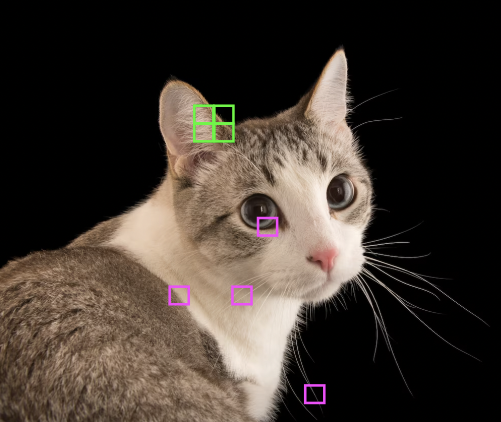
Fig. 39 Nearby pixels combine to form meaningful features of an image. Source
Let \(\boldsymbol{\mathsf X}\) be an \(n \times n\) input image and \(\boldsymbol{\mathsf{S}}\) be the \(m \times m\) output feature map. The banded weight matrix reduces the nonzero entries of the weight matrix from \(m^2 n^2\) to \(m^2{k}^2\) where a local region of \(k \times k\) pixels in the input image are mixed. If the feature detector is translationally invariant across the image, then the weights in each band are shared. This further reduces the number of weights to \(O(k^2).\) The resulting linear operation is called a convolution in two spatial dimensions:
Observe that spatial ordering of the pixels in the input \(\boldsymbol{\mathsf X}\) is preserved in the output \(\boldsymbol{\mathsf{S}}.\) This is nice since we want spatial information and orientation across a stack of convolution operations to be passed down into the final output.
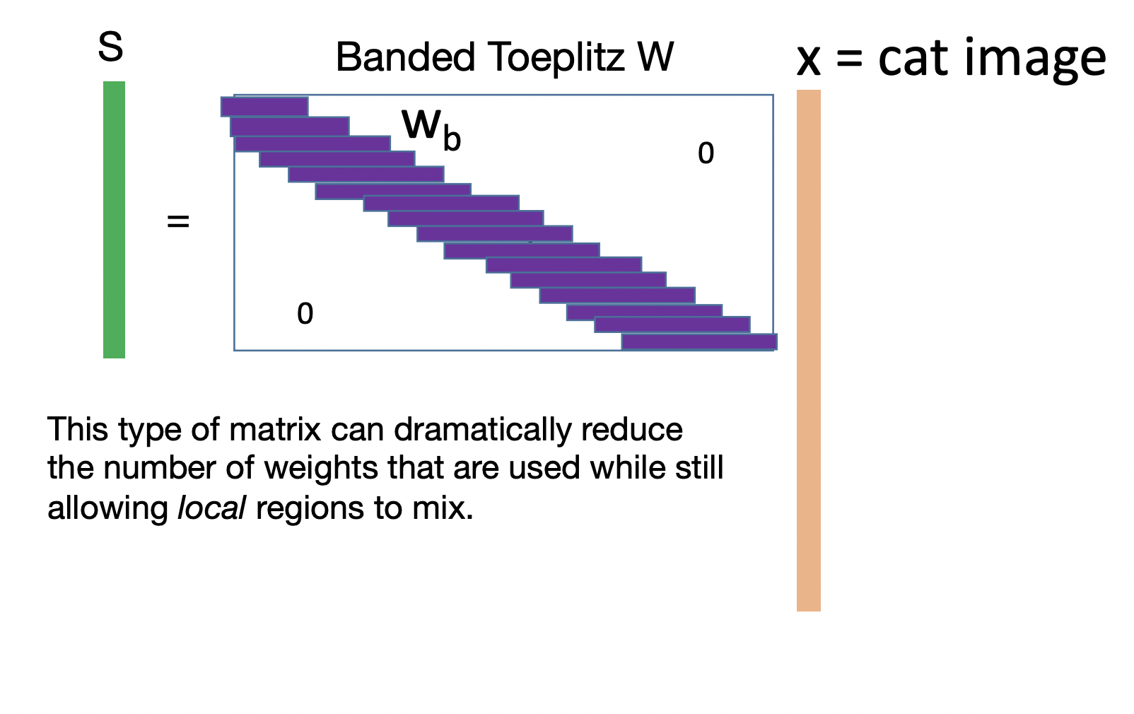
Fig. 40 Banded Toeplitz matrix for classifying cat images [Source]. The horizontal vectors contain the same pixel values. Note that there can be multiple bands for a 2D kernel. See this SO answer.
Remark. It can be shown that convolution has translation equivariance due to weight sharing.
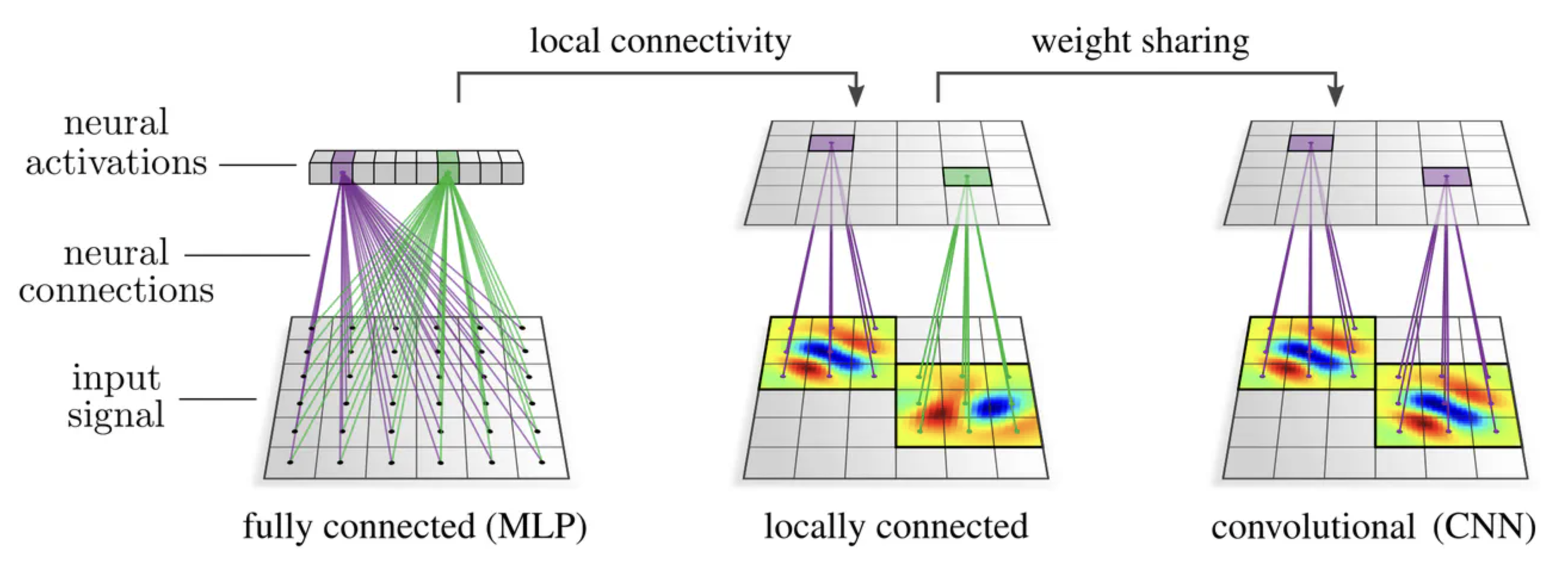
Fig. 41 Having local neural connectivity and weight sharing (both kernel and bias weights) characterizes the convolution. Source