Appendix: Guided Backprop

To explain the outputs of convolutional networks, we can look at the effect of each pixel in the input on each output node corresponding to a class. That is, we consider gradients \(\partial y / {\partial \boldsymbol{\mathsf{X}}^{\ell}}_{ij}\) for a target class \(y\) where \(\ell = 0\) for the input image. Note that gradients can be negative in intermediate layers, so to get a stronger signal we mask these gradients when computing backpropagation with respect to \({\boldsymbol{\mathsf{X}}^0}_{ij}\). In effect, we backpropagate only through those neurons which cause a first-order increase in the target class \(y\).

Moreover, positive activation indicate pattern detection for each node, hence we mask out nodes with negative activations further strengthening the signal. Since this is applied to all layers, we get patterns which are compositional and would eventually result in a positive activation for the target node. The gradients on input pixels are calculated with these two masks in place. This method is called Guided Backpropagation (GB) [SDBR14] used to obtain fine-grained details in the input image that contribute to the target class.

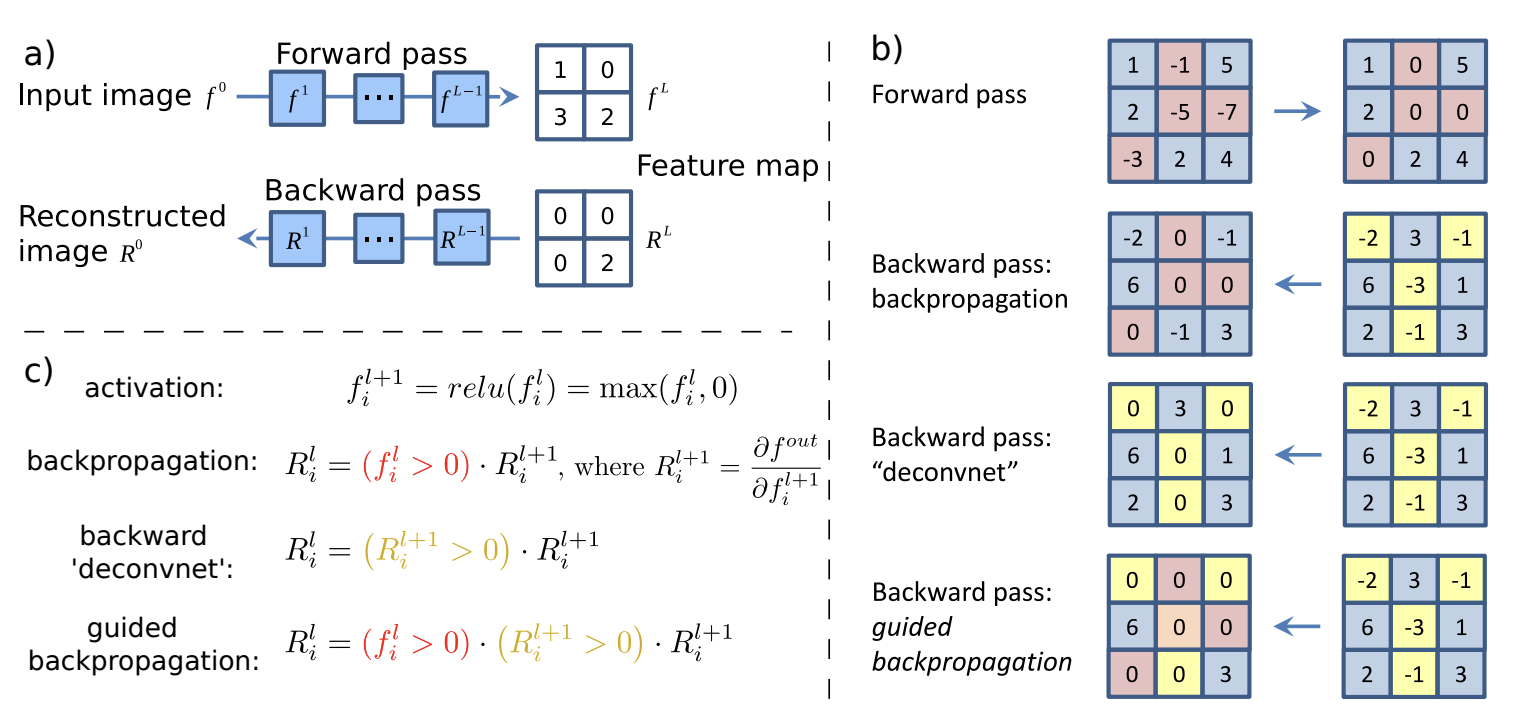
../../../_images/03-guided_backprop.png — Fig. 49 Schematic of visualizing the activations of high layer neurons. Source: Fig. 1 of [SDBR14]

def standardize_and_clip(x, min_val=0.0, max_val=1.0, saturation=0.1, brightness=0.5):
    x = x.detach().cpu()
    u = x.mean()
    v = max(x.std(), 1e-7)
    standardized = x.sub(u).div(v).mul(saturation)
    clipped = standardized.add(brightness).clamp(min_val, max_val)
    return clipped

def relu_hook_function(module, grad_in, grad_out):
    # Mask out negative gradients, and negative outputs
    # Note: ∂relu(x)/∂x = [x > 0] = [relu(x) > 0], 
    # so that ∂(relu input) = [relu(x) > 0] * ∂(relu output).
    # This explains why we take the gradient wrt relu input.
    return (torch.clamp(grad_in[0], min=0.),)

def resize(x):
    return transforms.Resize(size=(224, 224))(x)

def register_hooks(model):
    hooks = []
    for _, module in model.named_modules():
        if isinstance(module, torch.nn.ReLU):
            h = module.register_backward_hook(relu_hook_function)
            hooks.append(h)
    return hooks

def guided_backprop(model, x, target=None):
    hooks = register_hooks(model)

    # backward through target node
    with eval_context(model):
        p = model(x)
        if target is None:
            target = p.argmax().item()

        y = p[0, target]
        y.backward()

    g = standardize_and_clip(x.grad)
    g = g.to("cpu")
    x = x.to("cpu")
    
    # cleanup (gradients and hooks)
    for _, module in model.named_modules():
        module.zero_grad()

    for h in hooks:
        h.remove()

    return {
        "x": resize(x[0]),
        "g": resize(g[0]).max(dim=0)[0],    # <- max guided backprop! [1, H, W] map.
        "p": F.softmax(p, dim=1)[0, target]
    }   


# viz pathological tissue samples
outs = {}
target = 1
num_samples = 3
for b in range(num_samples):
    
    # prepare input image
    filepath = "data/histopathologic-cancer-detection/train"
    filename = data[data.label == target].iloc[b, 0]
    image = f"{filepath}/{filename}.tif"
    x = transform_infer(cv2.imread(image)).unsqueeze(0).to(DEVICE)
    x.requires_grad = True
    
    # magic happening...
    outs[b] = guided_backprop(model, x, target)

Remark. The backward hooks for masking negative gradients are only attached to ReLU layers since the network only has ReLU activations. See comments in the code. For other activations, you may need to implement forward hooks to mask out negative activations. See this video on PyTorch hooks for an introduction. 💡

Note that backward hooks are executed before the tensor saves its gradients. Moreover, its return value modifies the input gradients of the given module. Finally, we take the maximum for each input image channel to get a grayscale map for the gradients.

def normalize(x):
    """Map pixels to [0, 1]."""
    return (x - x.min()) / (x.max() - x.min())

# these can be sliders in a viz. app
min_val = 0.5
max_val = 10.0
overlay_alpha = 0.75

../../../_images/09e4ce3038950e05371c0450b16f29a744b1d05810bc351dd3f2035fe65b9889.svg

Not a domain expert on histopathology, but an expert on dog recognition. Let us compare how this looks like with pretrained AlexNet on a dog image:

transform = transforms.Compose([
    transforms.ToTensor(),
    transforms.Resize(224),
    transforms.CenterCrop(224),
    transforms.Normalize([0.485, 0.456, 0.406], [0.229, 0.224, 0.225])
])

image = cv2.imread("./data/shorty.png")
x = transform(image).unsqueeze(0).to(DEVICE)
x.requires_grad = True

alexnet = models.alexnet(pretrained=True).to(DEVICE)
out = guided_backprop(alexnet, x, target=None)

../../../_images/e921412afda101df7c7ce901fc3e261e1720e737eabd2454e57e4c0142adbb07.svg

Remark. It’s interesting that the model can pick out whiskers from the input image.