Negative log loss / MLE

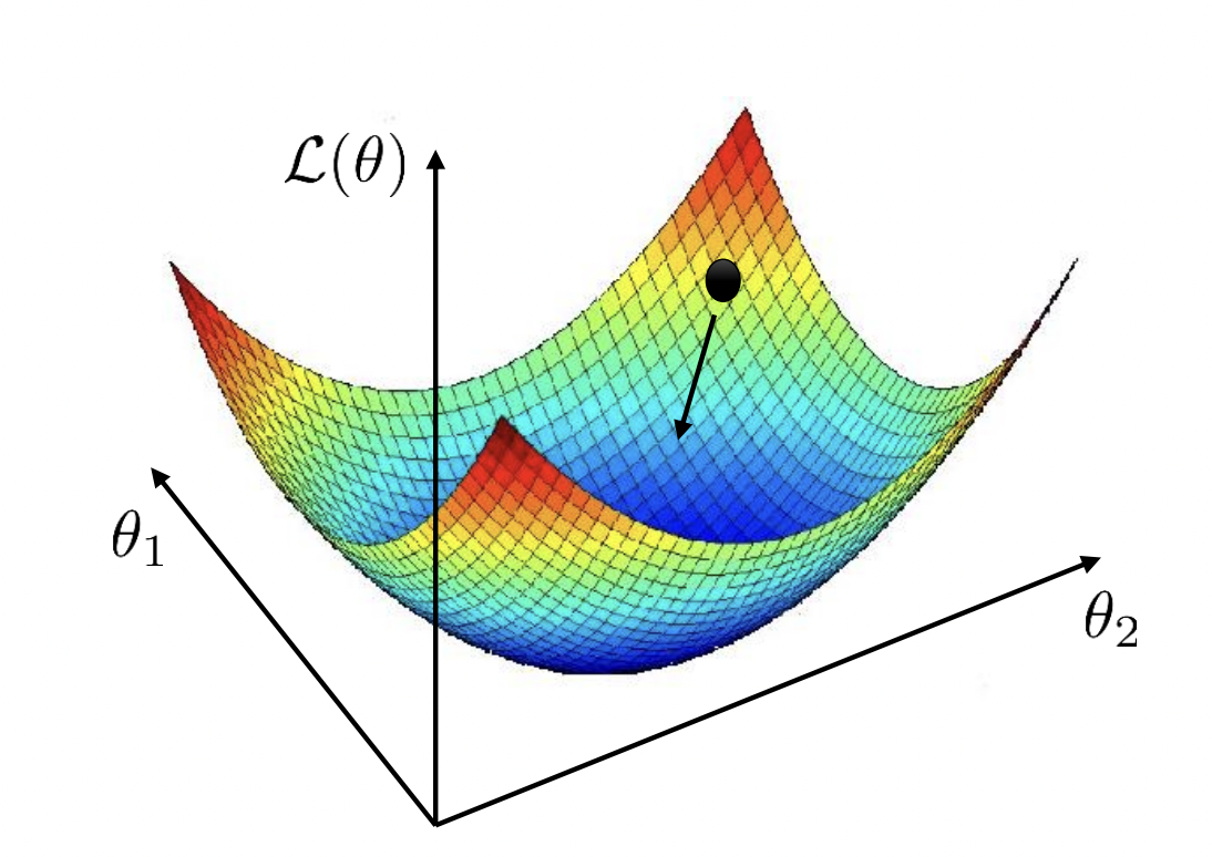
Machine learning training requires four steps: defining a model, defining a loss function, choosing an optimizer, and running it on large compute (e.g. GPUs). A loss function acts a smooth surrogate to the true objective which may not be amenable to available optimization techniques. Hence, we can think of loss functions as a measure of model quality. The choice of loss function determines what the model parameters will optimize towards.

Fig. 6 Loss surface for a model with two weights. Source

Here we derive a loss function based on the principle of maximum likelihood estimation (MLE), i.e. finding optimal parameters \(\hat{\boldsymbol{\Theta}}\) such that the dataset is assigned the highest probability under \(\hat{\boldsymbol{\Theta}}.\) Consider a parametric model of the target denoted by \(p_{\boldsymbol{\Theta}}(y \mid \boldsymbol{\mathsf{x}}).\) The likelihood of the IID sample \(\mathcal{D} = \{(\boldsymbol{\mathsf{x}}_i, y_i)\}_{i=1}^N\) can be defined as

\[ \begin{aligned} L(\boldsymbol{\Theta}) = \left({\prod_{i=1}^N {p_{\boldsymbol{\Theta}}(y_i \mid \boldsymbol{\mathsf{x}}_i)}}\right)^{\frac{1}{N}}. \end{aligned} \]

This is proportional to the probability assigned by the parametric model with parameters \(\boldsymbol{\Theta}\) on the sample \(\mathcal{D}.\) The IID assumption is important. Note that maximizing the likelihood results in a model that focuses more on inputs that are more probable since they are better represented in the sample. Probabilities are small numbers in \([0, 1]\), so applying the logarithm to convert the large product to a sum is a good idea:

\[ \begin{aligned} \log L(\boldsymbol{\Theta}) &= \frac{1}{N}\sum_{i=1}^N \log p_{\boldsymbol{\Theta}}(y_i \mid \boldsymbol{\mathsf{x}}_i). \end{aligned} \]

MLE then maximizes the log-likelihood with respect to the parameters \(\boldsymbol{\Theta}.\) The idea is that a good model makes training data more probable. It is customary in machine learning to convert this to a minimization problem. The following then becomes our optimization problem:

\[\hat{\boldsymbol{\Theta}} = \underset{\boldsymbol{\Theta}}{\text{argmin}}\,\left( -\frac{1}{N}\sum_{i=1}^N \log p_{\boldsymbol{\Theta}}(y_i \mid \boldsymbol{\mathsf{x}}_i)\right).\]

This allows us to define \(\ell = -\log p_{\boldsymbol{\Theta}}(y \mid \boldsymbol{\mathsf{x}}).\) In general, the loss function can be any nonnegative function whose value approaches zero whenever the prediction of the network the target value. Observe that:

• \(p_{\boldsymbol{\Theta}}(y \mid \boldsymbol{\mathsf{x}}) \to 1\) \(\implies\) \(\ell \to 0\)

• \(p_{\boldsymbol{\Theta}}(y \mid \boldsymbol{\mathsf{x}}) \to 0\) \(\implies\) \(\ell \to \infty\)

Using an expectation over the underlying distribution allows the model to focus on errors based on its probability of occuring. For every set of parameters \(\boldsymbol{\Theta},\) we approximate the true risk which is the expectation of \(\ell\) on the underlying distribution with the empirical risk calculated on the sample \(\mathcal{D}\):

\[\begin{split} \begin{aligned} \mathcal{L}(\boldsymbol{\Theta}) &= \mathbb{E}_{\boldsymbol{\mathsf{x}},y}\left[\ell(y, f_{\boldsymbol{\Theta}}(\boldsymbol{\mathsf{x}}))\right] \\ &\approx \frac{1}{|\mathcal{D}|} \sum_i \ell(y_i, f_{\boldsymbol{\Theta}}(\boldsymbol{\mathsf{x}}_i)) = \mathcal{L}_\mathcal{D}(\boldsymbol{\Theta}). \end{aligned} \end{split}\]

The optimization problem can be written more generally as \(\hat{\boldsymbol{\Theta}} = \underset{\boldsymbol{\Theta}}{\text{argmin}}\, \mathcal{L}_\mathcal{D}(\boldsymbol{\Theta}) \).

Cross-entropy

Note that the same input \({\boldsymbol{\mathsf{x}}}\) can have multiple labels in the dataset. Consider the contribution \(\mathcal{L}_{\boldsymbol{\mathsf{x}}}\) to the loss of the model’s predictions \(\hat{{p}}_{\boldsymbol{\mathsf{x}}} \in [0, 1]^C\) on an input \(\boldsymbol{\mathsf{x}}.\) Suppose each label has occured \(n^1, \ldots, n^C\) times given input \({\boldsymbol{\mathsf{x}}}\) out of \(N\) training pairs. Let \(n = n^1 + \ldots, n^C.\) Then,

\[\begin{split} \begin{aligned} \mathcal{L}_{\boldsymbol{\mathsf{x}}} &= -\frac{1}{N} \, \Big(n^1 \log \hat{{p}}_{\boldsymbol{\mathsf{x}}}^1 + \ldots + n^C \log \hat{{p}}_{\boldsymbol{\mathsf{x}}}^C \Big)\\ &= \frac{1}{N} \, \left[n^1, \ldots, n^C \right] \cdot -\log \hat{{p}}_{\boldsymbol{\mathsf{x}}} \\ &= \frac{n}{N} \, {\left[\frac{n^1}{n}, \ldots, \frac{n^C}{n}\right]} \cdot -\log \hat{{p}}_{\boldsymbol{\mathsf{x}}}. \end{aligned} \end{split}\]

Note that the dot product is the cross-entropy between[1] model predict probabilities and the label distribution[2] given input \(\boldsymbol{\mathsf{x}}.\) Finally, this cross-entropy is weighted by the empirical probability of \(\boldsymbol{\mathsf{x}}\) occuring. It follows that the NLL is equivalent to the expected cross-entropy between the model predict probabilities and the label distribution given an input. Consequently, any classification model trained to minimize cross-entropy on hard labels maximizes the likelihood of the training dataset.

Example. The PyTorch implementation of F.cross_entropy converts logits to probabilities using the softmax. Consistent with the above discussion, we can either pass hard labels \((B,)\) for a batch of \(B\) inputs, or \((B, C)\) where \(p_{ij} \in [0, 1]\) containing probabilities for class \(j\) (soft labels) given instance \(i.\)

import torch
import torch.nn.functional as F

s = torch.tensor([
    [0.3333, 0.3333, 0.3333],
    [0.3333, 0.3333, 0.3333],
    [0.3333, 0.3333, 0.3333],
    [0.4333, 0.2333, 0.3333],
    [0.3333, 0.2333, 0.4333],
    [0.1333, 0.3333, 0.5333],
])
y = torch.tensor([0, 1, 1, 0, 1, 2])
F.cross_entropy(s, target=y)         # expects logits -> applies softmax

tensor(1.0686)

F.cross_entropy calculates cross-entropy with softmax probas:

q = F.softmax(s, dim=1)
-torch.log(q[range(s.shape[0]), y]).mean()

tensor(1.0686)

Following the above discussion, we can also use soft labels based on empirical label distribution:

p = torch.tensor([
    [0.3333, 0.6666, 0.0000],
    [0.3333, 0.6666, 0.0000],
    [0.3333, 0.6666, 0.0000],
    [1.0000, 0.0000, 0.0000],
    [0.0000, 1.0000, 0.0000],
    [0.0000, 0.0000, 1.0000]
])

F.cross_entropy(s, target=p)

tensor(1.0685)

Or with one-hot probability vectors:

p = torch.tensor([
    [1.0000, 0.0000, 0.0000],
    [0.0000, 1.0000, 0.0000],
    [0.0000, 1.0000, 0.0000],
    [1.0000, 0.0000, 0.0000],
    [0.0000, 1.0000, 0.0000],
    [0.0000, 0.0000, 1.0000]
])

F.cross_entropy(s, target=p)

tensor(1.0686)

---

[1]

From Gibbs’ inequality, we have \(H(p, q) \geq H(p, p)\). Hence, the cross-entropy is minimized when the model predict probabilities precisely match the label distribution. In principle, the cross entropy measures the amount of “information” needed to describe outputs of the model. Recall that the input output pairs \((\boldsymbol{\mathsf{x}}, y)\) are generated by a random process. The cross entropy increases as more information is needed to describe each outcome of this random process.

[2]

The empirical label distribution becomes a one-hot vector whenever \(n = 1.\) In fact, we can convert each instance to a one-hot vector and calculate the loss as the expected cross-entropy with one-hot vectors as label distribution, even when an instance has multiple labels in the dataset, and get the same result. But deriving the probability distribution of the next state is important to understand as it occurs in a lot of scenarios (e.g. language modeling and RL).