Bidirectional Recurrent Units

For language modeling, i.e. predicting the next token, it makes sense to condition on the leftward context. However, it also makes sense to look at words from the right to fully understand a sentence. For example, a common task[1] is to mask out random tokens in a text document and then to train a sequence model to predict the values of the missing tokens. Depending on what comes after the blank, the likely value of the missing token changes dramatically:

I am ___.
I am ___ tired.
I am ___ tired, and I can sleep all day.

Clearly the meaning change by reading more into the sentence. The likely candidates change (e.g. “happy”, “not”, and “very” ), even when the tokens on the left of the blank are the same. Note that bidirectional RNNs typically only used in the encoding part of a system[2] since the rightward context is not available at inference.

Bidirectional computation

A simple technique transforms any RNN unit (e.g. LSTM, GRU) into a bidirectional unit [SP97]. The input sequence is simply processed in opposing directions. Then, outputs for the same inputs are concatenated for downstream processing. The states are processed independently in the expected order.

More precisely, let \(G\) be a recurrent unit. For \(t = 1, \ldots, T\), the forward direction computes:

\[ \boldsymbol{\mathsf{O}}^f_t, \boldsymbol{\mathsf{H}}^f_t = G(\boldsymbol{\mathsf{X}}_t, \boldsymbol{\mathsf{H}}^f_{t-1}) \]

Meanwhile, the backward direction calculates:

\[ \boldsymbol{\mathsf{O}}^b_{T - t + 1}, \boldsymbol{\mathsf{H}}^b_t = G(\boldsymbol{\mathsf{X}}_{T - t + 1}, \boldsymbol{\mathsf{H}}^b_{t-1}) \]

Finally, the output sequence is given by

\[(\boldsymbol{\mathsf{O}}^f_t \oplus \boldsymbol{\mathsf{O}}^b_t)_{t=1}^T.\]

Note that input indices have to be matched. This is illustrated in Fig. 64.

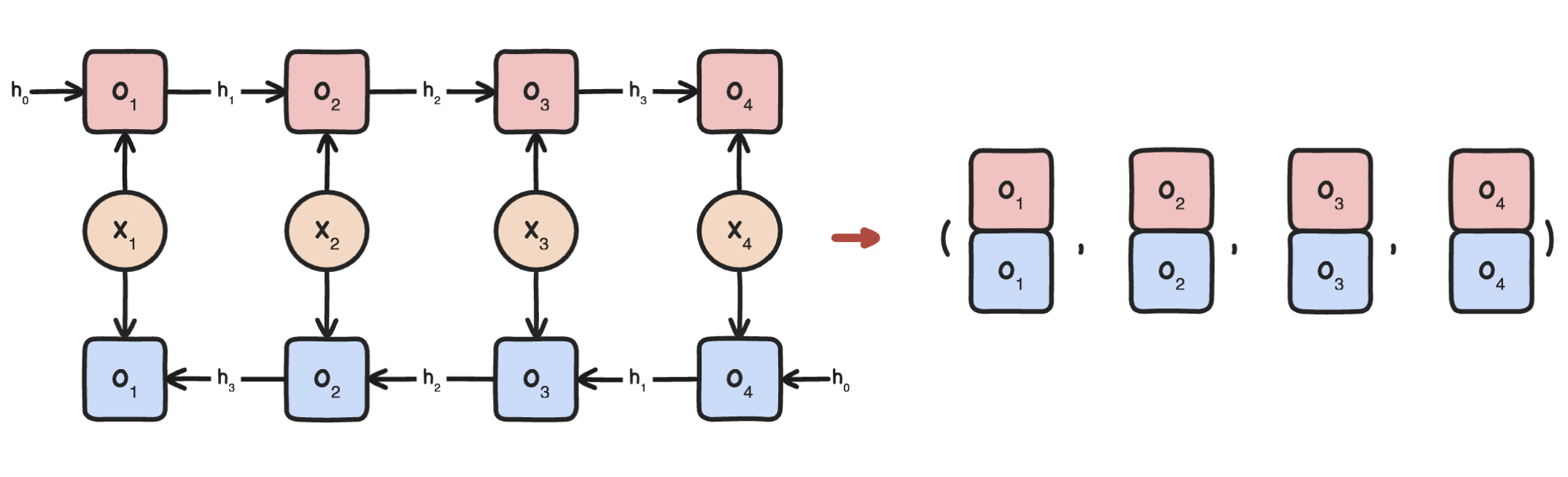
Fig. 64 Building the output vectors (right) in a bidirectional recurrent computation.

Code implementation

Creating a Bidirectional wrapper unit to convert any to a bidirectional RNN cell:

from functools import partial

class BiRNN(RNNBase):
    def __init__(self, 
        cell: Type[RNNBase],
        inputs_dim: int, hidden_dim: int, 
        **kwargs
    ):
        super().__init__(inputs_dim, hidden_dim)
        assert hidden_dim % 2 == 0
        self.frnn = cell(inputs_dim, hidden_dim // 2, **kwargs)
        self.brnn = cell(inputs_dim, hidden_dim // 2, **kwargs)
        
    def init_state(self, x):
        return (None, None)

    def compute(self, x, state):
        fh, bh = state
        fo, fh = self.frnn(x, fh)
        bo, bh = self.brnn(torch.flip(x, [0]), bh)  # Flip seq index: (T, B, d)
        bo = torch.flip(bo, [0])                    # Flip back outputs. See above
        outs = torch.cat([fo, bo], dim=-1)
        return outs, (fh, bh)


Bidirectional = lambda cell: partial(BiRNN, cell)

Remark. For consistency with LanguageModel, we expect that the hidden_dim parameter is the size of the combined forward and backward outputs. This is so that the linear layer matches the given parameter. In other words, we halve the hidden size of each RNN cell inside the bidirectional model.

Flip function works as follows:

l = [[i, 2 * i] for i in range(6)]
a = torch.tensor(l).reshape(-1, 3, 2)
a

tensor([[[ 0,  0],
         [ 1,  2],
         [ 2,  4]],

        [[ 3,  6],
         [ 4,  8],
         [ 5, 10]]])

Only time dimension is affected by flip:

torch.flip(a, [0])

tensor([[[ 3,  6],
         [ 4,  8],
         [ 5, 10]],

        [[ 0,  0],
         [ 1,  2],
         [ 2,  4]]])

Shapes. Recall LSTM has two states. And one state vector for each input sequence:

blstm = Bidirectional(LSTM)(28, 128)
x = torch.randn(30, 32, 28)
outs, (fstate, bstate) = blstm(x)
assert outs.shape == (30, 32, 128)
assert fstate[0].shape == (32, 64), fstate[1].shape == (32, 64)
assert bstate[0].shape == (32, 64), bstate[1].shape == (32, 64)

Our implementation differs a bit with PyTorch where hidden size is doubled:

blstm_torch = nn.LSTM(28, 64, bidirectional=True)
for net in [blstm, blstm_torch]:
    for name, p in net.named_parameters():
        if "bias" in name:
            p.data.fill_(0.0)
        else:
            p.data.fill_(1.0)

error = torch.abs(blstm(x)[0] - blstm_torch(x)[0]).max()
print(error)
assert error < 5e-6

tensor(1.1176e-06, grad_fn=<MaxBackward1>)

Adding depth still works:

blstm = Deep(Bidirectional(LSTM))(28, 128, num_layers=2)
blstm_torch = nn.LSTM(28, 64, bidirectional=True, num_layers=2)
for net in [blstm, blstm_torch]:
    for name, p in net.named_parameters():
        if "bias" in name:
            p.data.fill_(0.0)
        else:
            p.data.fill_(1.0)

error = torch.abs(blstm(x)[0] - blstm_torch(x)[0]).max()
print(error)
assert error < 1e-5

tensor(0., grad_fn=<MaxBackward1>)

Remark. Bidirectional first, then deep. We will train such a model below. This allows each layer to benefit from the bidirectional context before passing it to the next layer, i.e. the higher-order states also look at the previous states in two directions. The zero error above shows that this setup is consistent with the PyTorch implementation.

Model training

Demo. Training a BiLSTM based sentiment classifier on the IMDB movie review dataset:

import keras
import torch
from torch.utils.data import TensorDataset, DataLoader

def collate_fn(batch):
    """Transforming the data to sequence-first format."""
    x, y = zip(*batch)
    x = torch.stack(x, 1)      # (T, B)
    y = torch.stack(y, 0)      # (B,)
    return x, y


BATCH_SIZE = 16
MAX_WORDS = 20_000          # Only top MAX_WORDS words, else <unk>
T = 256                     # Only read T words of each movie review
PADDING_IDX = MAX_WORDS     # In practice, 0 may be <unk>, so new idx for padding

# Load. Trim or pad sequences to length T
(x_train, y_train), (x_valid, y_valid) = keras.datasets.imdb.load_data(num_words=MAX_WORDS)
x_train = keras.utils.pad_sequences(x_train, maxlen=T, value=PADDING_IDX)
x_valid = keras.utils.pad_sequences(x_valid, maxlen=T, value=PADDING_IDX)
print(x_train.shape, x_valid.shape)

train_dataset = TensorDataset(torch.tensor(x_train), torch.tensor(y_train).long())
valid_dataset = TensorDataset(torch.tensor(x_valid), torch.tensor(y_valid).long())
train_loader = DataLoader(train_dataset, batch_size=BATCH_SIZE, shuffle=True, collate_fn=collate_fn)
valid_loader = DataLoader(valid_dataset, batch_size=BATCH_SIZE, shuffle=True, collate_fn=collate_fn)    # also sampled

(25000, 256) (25000, 256)

import numpy as np
import matplotlib.pyplot as plt
from matplotlib_inline import backend_inline
backend_inline.set_matplotlib_formats("svg")

x = np.log(x_train[0] + 1)
plt.imshow(((x - x.min()) / (x.max() - x.min())).reshape(8, 32));

Observe that the sequence is pre-padded, i.e. padding token is added from the left[3]. This is good so that padding elements are processed before the RNN internal states are updated with information from actual inputs. Of course, it would be better if the RNN explicitly ignores the padding element (for efficiency). Later it will be shown that LSTM networks and GRU are able to effectively ignore the padding vector during training.

from tqdm.notebook import tqdm

def train_step(model, optim, x, y, max_norm) -> float:
    loss = F.cross_entropy(model(x), y)
    loss.backward()
    
    model[0].weight.grad[PADDING_IDX] = 0.0
    clip_grad_norm(model, max_norm=max_norm)
    optim.step()
    optim.zero_grad()

    return loss.item()
 
@torch.no_grad()
def valid_step(model, x, y) -> float:
    loss = F.cross_entropy(model(x), y)
    return loss.item()

class LastElement(nn.Module):
    """Get last element of a rank-3 tensor of shape (T, B, h)."""
    def forward(self, x):
        return x[0][-1]


DEVICE = "mps"
LR = 1e-4
EPOCHS = 3
MAX_NORM = 5.0
EMBED_DIM = 512
HIDDEN_DIM = 128

emb = nn.Embedding(MAX_WORDS + 1, EMBED_DIM, padding_idx=PADDING_IDX)
rnn = Deep(Bidirectional(nn.LSTM))(EMBED_DIM, HIDDEN_DIM, num_layers=3, bias=False)
model = nn.Sequential(
    emb, rnn, LastElement(),
    nn.Dropout(0.2),
    nn.Linear(HIDDEN_DIM, 2)
)
model = model.to(DEVICE)
optim = torch.optim.Adam(model.parameters(), lr=LR)

train_loss = []
valid_loss = []
valid_accs = []

for e in tqdm(range(EPOCHS)):
    for t, (x, y) in tqdm(enumerate(train_loader), total=len(train_loader)):
        x = x.to(DEVICE)
        y = y.to(DEVICE)
        loss = train_step(model, optim, x, y, MAX_NORM)
        train_loss.append(loss)

        if t % 5 == 0:
            xv, yv = next(iter(valid_loader))
            xv = xv.to(DEVICE)
            yv = yv.to(DEVICE)
            valid_loss.append(valid_step(model, xv, yv))
            valid_accs.append((model(xv).argmax(dim=1) == yv).float().mean().item())

Remark. Setting padding_idx in nn.Embedding makes the embedding vector for the padding token zero. Moreover, we set bias=False in the RNN. These constraints stabilized network training since the LSTM unit (also GRU) will have zero output for a sequence of padding tokens of any length[4]. This is consistent with adding the padding tokens to the left, so that network output is unaffected by the amount of left padding. Finally, gradients are leaking to the padding token due to BPTT, so we use the ff. heuristic to keep the padding embedding fixed:

model[0].weight.grad[PADDING_IDX] = 0.0

Evaluating validation accuracy:

c = 0
for xv, yv in tqdm(valid_loader):
    xv = xv.to(DEVICE)
    yv = yv.to(DEVICE)
    c += (model(xv).argmax(dim=1) == yv).int().sum().item()

print(c / len(valid_dataset))

0.87212

Show code cell source Hide code cell source

fig, ax1 = plt.subplots(figsize=(6, 4))

WINDOW_SIZE = int(0.05 * len(valid_loss))
train_loss = np.array(train_loss)
valid_loss = np.array(valid_loss)
valid_accs = np.array(valid_accs)
train_loss_avg = [train_loss[i-WINDOW_SIZE * 5:i].mean() for i in range(WINDOW_SIZE * 5, len(train_loss))]
valid_loss_avg = [valid_loss[i-WINDOW_SIZE:i].mean() for i in range(WINDOW_SIZE, len(valid_loss))]
valid_accs_avg = [valid_accs[i-WINDOW_SIZE:i].mean() for i in range(WINDOW_SIZE, len(valid_accs))]

ax1.plot(train_loss_avg, linewidth=2, alpha=0.6, label="train loss", color="C0")
ax1.set_xlabel("step")
ax1.grid(axis="both", linestyle="dotted", alpha=0.8)
ax2 = ax1.twinx()
ax1.plot(np.array(range(1, len(valid_loss_avg) + 1)) * 5, valid_loss_avg, linewidth=2, label="valid loss", color="C0")
ax2.plot(np.array(range(1, len(valid_accs_avg) + 1)) * 5, valid_accs_avg, linewidth=2, label="valid accs", color="C1")

ax1.set_ylabel("loss", fontsize=10)
ax2.set_ylabel("accuracy", fontsize=10)
ax1.xaxis.set_label_coords(1.00, -0.020)
ax1.legend(loc="lower right", fontsize=10)
ax2.legend(loc="upper right", fontsize=10)
ax2.legend(loc='upper center', bbox_to_anchor=(0.1, -0.10), ncol=5)
ax1.legend(loc='lower center', bbox_to_anchor=(0.8, -0.20), ncol=5);

Checking trained model outputs zero vector on padding tokens:

z = (torch.ones(256, 1).to(DEVICE) * PADDING_IDX).long()
out, state = model[1](model[0](z))

# forward is zero
error = (out.abs() - torch.zeros(256, 1, 128).to(DEVICE)).mean().item()
assert error == 0.0

# internal states are zero
for l in range(model[1].num_layers):
    (hf, cf), (hb, cb) = state[l]
    assert hf.sum() + cf.sum() == 0
    assert hb.sum() + cb.sum() == 0

---

[1]

Often useful for model pretraining prior to fine-tuning on an actual task of interest.

[2]

Encoding refers to ingesting an input sequence \(\boldsymbol{\mathsf{x}}\) to get a state vector \(\boldsymbol{\mathsf{h}}\) that, in principle, distills the relevant information in that sequence relative to the downstream task. For example, recall in text generation \(\boldsymbol{\mathsf{h}} = \text{RNN}(\boldsymbol{\mathsf{x}}_{\text{prompt}})\) is the encoding used to start the decoding process, i.e. using the state vector and the model’s generative capabilities to produce text.

[3]

RNNs can handle variable-length sequence inputs when \(B = 1.\) However, to efficiently process batches of input, we have to have batches with the same shape \((T, B, d)\) hence the same sequence length. One way to do this is to pack sequences, where variable sized batches are constructed based on sequences that still have elements, so that padding is effectively ignored by the network. See this SO answer.

[4]

This is an exact property of LSTM without bias: \(\tilde{\boldsymbol{\mathsf{C}}}_t=\tanh \left(\boldsymbol{\mathsf{X}}_t^{\text{emb}} \boldsymbol{\mathsf{U}^c}+\boldsymbol{\mathsf{H}}_{t-1} \boldsymbol{\mathsf{W}^c}\right) = \boldsymbol{0}\) whenever \(\boldsymbol{\mathsf{X}}_t^{\text{emb}} = \boldsymbol{0}\) and \(\boldsymbol{\mathsf{H}}_{t-1} = \boldsymbol{0}.\) Moreover, \({\boldsymbol{\mathsf{H}}}_t\) is also zero since it’s the gated \(\tanh\left( \boldsymbol{\mathsf{C}}_t \right)\) and \(\tanh 0 = 0.\) And because \(\boldsymbol{\mathsf{H}}_0 = \boldsymbol{0}\) and \(\boldsymbol{\mathsf{C}}_0 = \boldsymbol{0}\), the states do not update every time we get the padding token as input. By a similar calculation, the GRU can be shown to have this property.